https://www.giss.nasa.gov/tools/gprojector/help/projections/ https://freegeographytools.com/2007/online-map-projection-viewers-i [[Longitude]] [[Maps and the Coordinate Systems they are Projected From]] [[Library/Maps and the Coordinate Systems they are Projected From|Maps and the Coordinate Systems they are Projected From]] ky Miles]] [[Sky Mile Slide Deck]] [[The Sky Mile Presentation]] [[Sidereal Solar and Lunar Time]] [[Coordinate Systems]] [[Coordinate System and Map Projection Papers]] [[Longitude]] [[Maps and the Coordinate Systems they are Projected From]] [[Cosmography]] [[G Projector Map Software]] [[Attachments/Optics Derived .docx|Optics Derived ]] [[Optics Angular Resolution or Earth Curve]] [[Angular Resolution and our World]] [[Basic Trigonometry angular size, distance, and]] [[The Celestial Sphere]] [[69 Miles Per Degree]] ![[Attachments/Pasted image 20240315101656.png]] https://www.giss.nasa.gov/tools/gprojector/help/references.html ## G.Projector 3 — Map Projection Explorer ### User's Guide: List of Map Projections - [Tobler hyperelliptical](https://en.wikipedia.org/wiki/Tobler_hyperelliptical_projection "Tobler hyperelliptical projection") [](https://en.wikipedia.org/wiki/File:Tobler_hyperelliptical_projection_SW.jpg) - [Mollweide](https://en.wikipedia.org/wiki/Mollweide_projection "Mollweide projection") [](https://en.wikipedia.org/wiki/File:Mollweide_projection_SW.jpg) - [Goode homolosine](https://en.wikipedia.org/wiki/Goode_homolosine_projection "Goode homolosine projection") [](https://en.wikipedia.org/wiki/File:Goode_homolosine_projection_SW.jpg) - [Eckert IV](https://en.wikipedia.org/wiki/Eckert_IV_projection "Eckert IV projection") [](https://en.wikipedia.org/wiki/File:Ecker_IV_projection_SW.jpg) - [Eckert VI](https://en.wikipedia.org/wiki/Eckert_VI_projection "Eckert VI projection") [](https://en.wikipedia.org/wiki/File:Ecker_VI_projection_SW.jpg) - [Kavrayskiy VII](https://en.wikipedia.org/wiki/Kavrayskiy_VII_projection "Kavrayskiy VII projection") [](https://en.wikipedia.org/wiki/File:Kavraiskiy_VII_projection_SW.jpg) ![[Attachments/Pasted image 20240415043618.png]] ### Type of projection surface[[edit](https://en.wikipedia.org/w/index.php?title=List_of_map_projections&action=edit&section=3 "Edit section: Type of projection surface")] 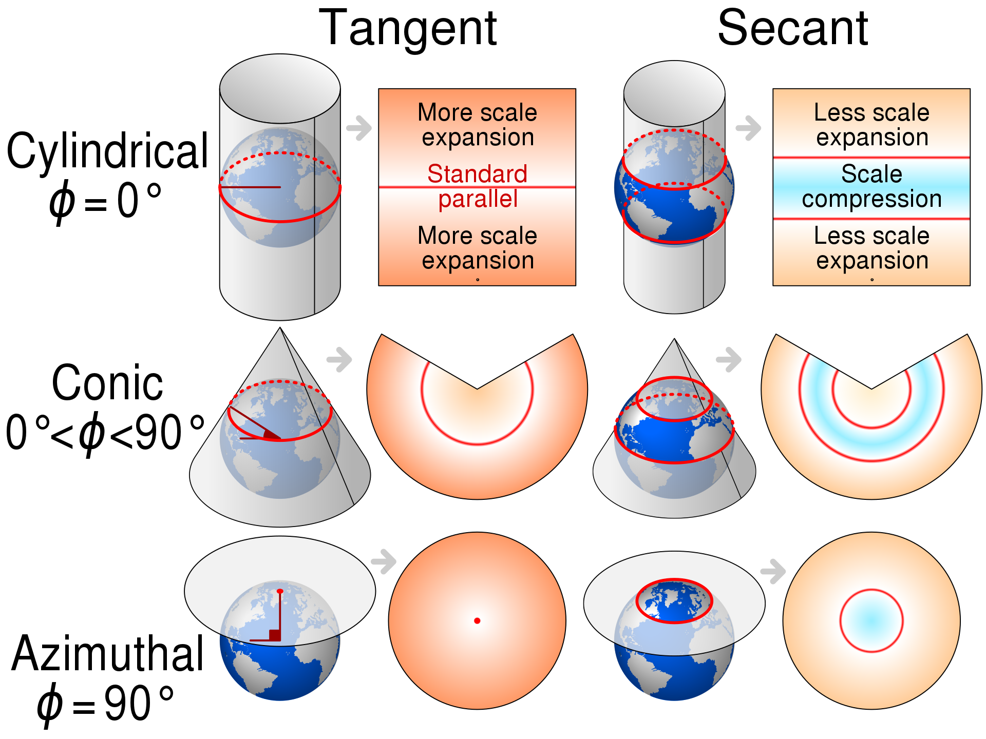Cylindrical In normal aspect, these map regularly-spaced meridians to equally spaced vertical lines, and parallels to horizontal lines. Pseudocylindrical In normal aspect, these map the central meridian and parallels as straight lines. Other meridians are curves (or possibly straight from pole to equator), regularly spaced along parallels. Conic In normal aspect, conic (or conical) projections map meridians as straight lines, and parallels as arcs of circles. Pseudoconical In normal aspect, pseudoconical projections represent the central meridian as a straight line, other meridians as complex curves, and parallels as circular arcs. Azimuthal In standard presentation, azimuthal projections map meridians as straight lines and parallels as complete, concentric circles. They are radially symmetrical. In any presentation (or aspect), they preserve directions from the center point. This means great circles through the central point are represented by straight lines on the map. Pseudoazimuthal In normal aspect, pseudoazimuthal projections map the equator and central meridian to perpendicular, intersecting straight lines. They map parallels to complex curves bowing away from the equator, and meridians to complex curves bowing in toward the central meridian. Listed here after pseudocylindrical as generally similar to them in shape and purpose. Other Typically calculated from formula, and not based on a particular projection Polyhedral maps Polyhedral maps can be folded up into a polyhedral approximation to the sphere, using particular projection to map each face with low distortion. ## Types Main article: [Equal-area projection](https://en.wikipedia.org/wiki/Equal-area_projection "Equal-area projection") [](https://en.wikipedia.org/wiki/File:Mollweide_projection_SW.jpg) The equal-area [Mollweide projection](https://en.wikipedia.org/wiki/Mollweide_projection "Mollweide projection") Equal-area maps preserve area measure, generally distorting shapes in order to do so. Equal-area maps are also called _equivalent_ or _authalic_. These are some projections that preserve area: - [Albers conic](https://en.wikipedia.org/wiki/Albers_conic_projection "Albers conic projection") - [Boggs eumorphic](https://en.wikipedia.org/wiki/Boggs_eumorphic_projection "Boggs eumorphic projection") - [Bonne](https://en.wikipedia.org/wiki/Bonne_projection "Bonne projection") - [Bottomley](https://en.wikipedia.org/wiki/Bottomley_projection "Bottomley projection") - [Collignon](https://en.wikipedia.org/wiki/Collignon_projection "Collignon projection") - [Cylindrical equal-area](https://en.wikipedia.org/wiki/Cylindrical_equal-area_projection "Cylindrical equal-area projection") - [Eckert II](https://en.wikipedia.org/wiki/Eckert_II_projection "Eckert II projection"), [IV](https://en.wikipedia.org/wiki/Eckert_IV_projection "Eckert IV projection") and [VI](https://en.wikipedia.org/wiki/Eckert_VI_projection "Eckert VI projection") - [Equal Earth](https://en.wikipedia.org/wiki/Equal_Earth_projection "Equal Earth projection") - [Gall orthographic](https://en.wikipedia.org/wiki/Gall%E2%80%93Peters_projection "Gall–Peters projection") (also known as Gall–Peters, or Peters, projection) - [Goode's homolosine](https://en.wikipedia.org/wiki/Goode_homolosine_projection "Goode homolosine projection") - [Hammer](https://en.wikipedia.org/wiki/Hammer_projection "Hammer projection") - [Hobo–Dyer](https://en.wikipedia.org/wiki/Hobo%E2%80%93Dyer_projection "Hobo–Dyer projection") - [Lambert azimuthal equal-area](https://en.wikipedia.org/wiki/Lambert_azimuthal_equal-area_projection "Lambert azimuthal equal-area projection") - [Lambert cylindrical equal-area](https://en.wikipedia.org/wiki/Lambert_cylindrical_equal-area_projection "Lambert cylindrical equal-area projection") - [Mollweide](https://en.wikipedia.org/wiki/Mollweide_projection "Mollweide projection") - [Sinusoidal](https://en.wikipedia.org/wiki/Sinusoidal_projection "Sinusoidal projection") - [Strebe 1995](https://en.wikipedia.org/wiki/Strebe_1995_projection "Strebe 1995 projection") - [Snyder's equal-area polyhedral projection](https://en.wikipedia.org/wiki/Snyder_equal-area_projection "Snyder equal-area projection"), used for [geodesic grids](https://en.wikipedia.org/wiki/Geodesic_grid "Geodesic grid"). - [Tobler hyperelliptical](https://en.wikipedia.org/wiki/Tobler_hyperelliptical_projection "Tobler hyperelliptical projection") - [Werner](https://en.wikipedia.org/wiki/Werner_projection "Werner projection") ### Equidistant [](https://en.wikipedia.org/wiki/File:Two-point_equidistant_projection_SW.jpg) A [two-point equidistant projection](https://en.wikipedia.org/wiki/Two-point_equidistant_projection "Two-point equidistant projection") of Eurasia If the length of the line segment connecting two projected points on the plane is proportional to the geodesic (shortest surface) distance between the two unprojected points on the globe, then we say that distance has been preserved between those two points. An **equidistant projection** preserves distances from one or two special points to all other points. The special point or points may get stretched into a line or curve segment when projected. In that case, the point on the line or curve segment closest to the point being measured to must be used to measure the distance. - [Plate carrée](https://en.wikipedia.org/wiki/Plate_carr%C3%A9e_projection "Plate carrée projection"): Distances from the two poles are preserved, in equatorial aspect. - [Azimuthal equidistant](https://en.wikipedia.org/wiki/Azimuthal_equidistant_projection "Azimuthal equidistant projection"): Distances from the center and edge are preserved. - [Equidistant conic](https://en.wikipedia.org/wiki/Equidistant_conic_projection "Equidistant conic projection"): Distances from the two poles are preserved, in equatorial aspect. - [Werner cordiform](https://en.wikipedia.org/wiki/Werner_cordiform_projection "Werner cordiform projection") Distances from the [North Pole](https://en.wikipedia.org/wiki/North_Pole "North Pole") are preserved, in equatorial aspect. - [Two-point equidistant](https://en.wikipedia.org/wiki/Two-point_equidistant_projection "Two-point equidistant projection"): Two "control points" are arbitrarily chosen by the map maker; distances from each control point are preserved. ### Gnomonic[ [](https://en.wikipedia.org/wiki/File:Usgs_map_gnomic.PNG) The [Gnomonic projection](https://en.wikipedia.org/wiki/Gnomonic_projection "Gnomonic projection") is thought to be the oldest map projection, developed by [Thales](https://en.wikipedia.org/wiki/Thales "Thales") in the 6th century BC [Great circles](https://en.wikipedia.org/wiki/Great_circle "Great circle") are displayed as straight lines: - [Gnomonic projection](https://en.wikipedia.org/wiki/Gnomonic_projection "Gnomonic projection") ### Retroazimuthal Direction to a fixed location B (the bearing at the starting location A of the shortest route) corresponds to the direction on the map from A to B: - [Littrow](https://en.wikipedia.org/wiki/Littrow_projection "Littrow projection")—the only conformal retroazimuthal projection - [Hammer retroazimuthal](https://en.wikipedia.org/wiki/Hammer_retroazimuthal_projection "Hammer retroazimuthal projection")—also preserves distance from the central point - [Craig retroazimuthal](https://en.wikipedia.org/wiki/Craig_retroazimuthal_projection "Craig retroazimuthal projection") _aka_ Mecca or Qibla—also has vertical meridians ### Compromise projections[] [](https://en.wikipedia.org/wiki/File:Usgs_map_robinson.PNG) The [Robinson projection](https://en.wikipedia.org/wiki/Robinson_projection "Robinson projection") was adopted by _[National Geographic](https://en.wikipedia.org/wiki/National_Geographic_(magazine) "National Geographic (magazine)")_ magazine in 1988 but abandoned by them in about 1997 for the [Winkel tripel](https://en.wikipedia.org/wiki/Winkel_tripel_projection "Winkel tripel projection"). Compromise projections give up the idea of perfectly preserving metric properties, seeking instead to strike a balance between distortions, or to simply make things look right. Most of these types of projections distort shape in the polar regions more than at the equator. These are some compromise projections: - [Robinson](https://en.wikipedia.org/wiki/Robinson_projection "Robinson projection") - [van der Grinten](https://en.wikipedia.org/wiki/Van_der_Grinten_projection "Van der Grinten projection") - [Miller cylindrical](https://en.wikipedia.org/wiki/Miller_cylindrical_projection "Miller cylindrical projection") - [Winkel Tripel](https://en.wikipedia.org/wiki/Winkel_tripel_projection "Winkel tripel projection") - [Buckminster Fuller's Dymaxion](https://en.wikipedia.org/wiki/Dymaxion_map "Dymaxion map") - [B. J. S. Cahill's Butterfly Map](https://en.wikipedia.org/wiki/Bernard_J._S._Cahill "Bernard J. S. Cahill") - [Kavrayskiy VII projection](https://en.wikipedia.org/wiki/Kavrayskiy_VII_projection "Kavrayskiy VII projection") - [Wagner VI projection](https://en.wikipedia.org/wiki/Wagner_VI_projection "Wagner VI projection") - [Chamberlin trimetric](https://en.wikipedia.org/wiki/Chamberlin_trimetric_projection "Chamberlin trimetric projection") - [Oronce Finé](https://en.wikipedia.org/wiki/Oronce_Fin%C3%A9 "Oronce Finé")'s cordiform - [AuthaGraph projection](https://en.wikipedia.org/wiki/AuthaGraph_projection "AuthaGraph projection") #### • Return ![[Attachments/Pasted image 20240415043431.png]] ## Table of projections] | Year | Projection | Image | Type | Properties | Creator | Notes | | ---------------- | ------------------------------------------------------------------------------------------------------------------------------------------------------------------------------------------------------------- | ---------------------------------------------------------------------------------------------------------------------------------------------------------------------------------------------------------------------------------------------------------------------- | ------------------------------------------------------------------------------------- | ----------------------- | --------------------------------------------------------------------------------------------------------------------------------------------------------------------------------------------------------------------------------------- | ------------------------------------------------------------------------------------------------------------------------------------------------------------------------------------------------------------------------------------------------------------------------------------------------------------------------------------------------------------------------------------------------------------------------------------------------------------------------------------------------------ | | c. 120 | [Equirectangular](https://en.wikipedia.org/wiki/Equirectangular_projection "Equirectangular projection") <br>= equidistant cylindrical <br>= rectangular <br>= la carte parallélogrammatique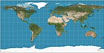 | [](https://en.wikipedia.org/wiki/File:Equirectangular_projection_SW.jpg) | Cylindrical | Equidistant | [Marinus of Tyre](https://en.wikipedia.org/wiki/Marinus_of_Tyre "Marinus of Tyre") | Simplest geometry; distances along meridians are conserved. <br><br>[Plate carrée](https://en.wikipedia.org/wiki/Plate_carr%C3%A9e_projection "Plate carrée projection"): special case having the equator as the standard parallel. | | 1745 | [Cassini](https://en.wikipedia.org/wiki/Cassini_projection "Cassini projection") <br>= Cassini–Soldner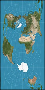 | [](https://en.wikipedia.org/wiki/File:Cassini_projection_SW.jpg) | Cylindrical | Equidistant | [César-François Cassini de Thury](https://en.wikipedia.org/wiki/C%C3%A9sar-Fran%C3%A7ois_Cassini_de_Thury "César-François Cassini de Thury") | Transverse of equidistant projection; distances along central meridian are conserved. <br>Distances perpendicular to central meridian are preserved. 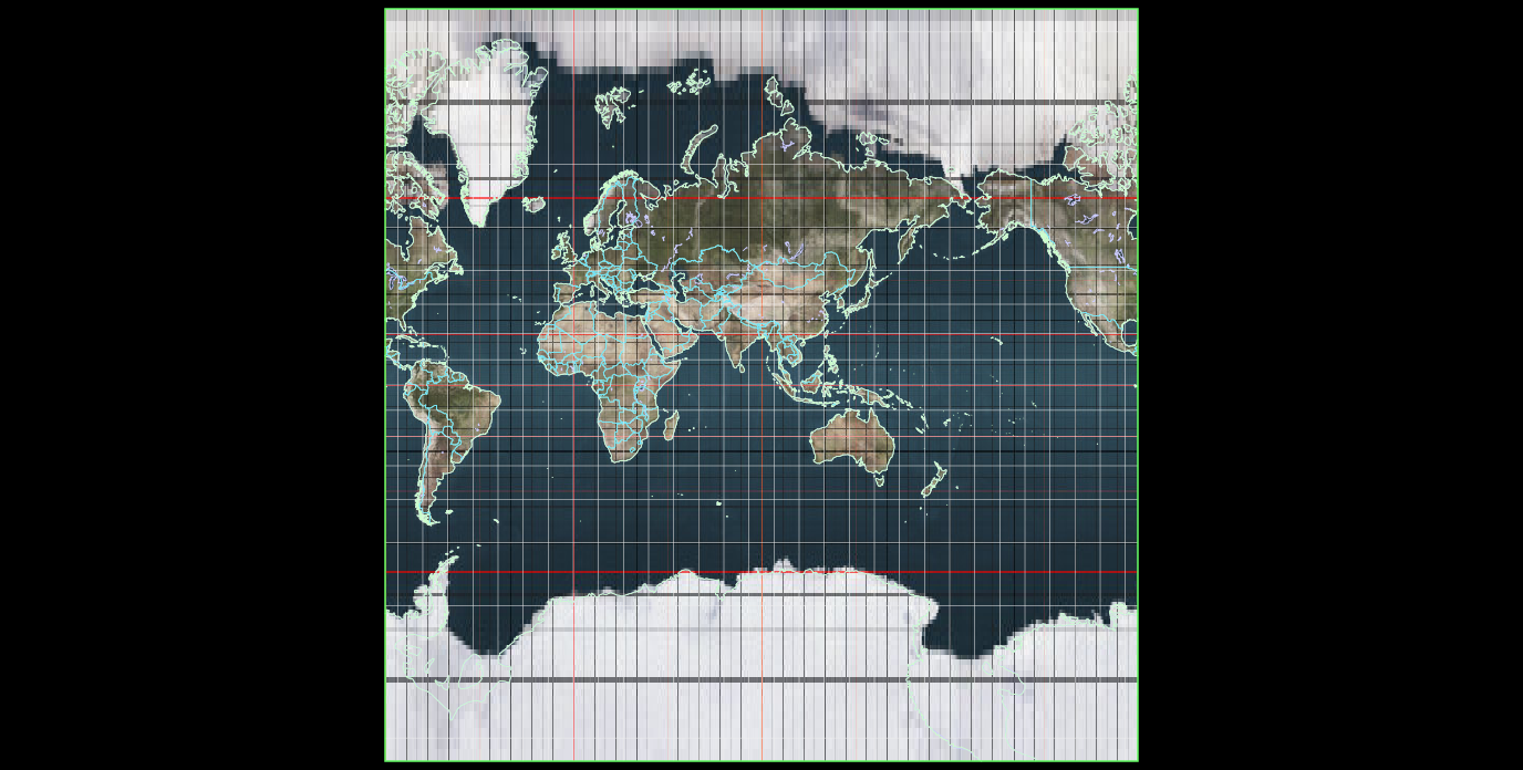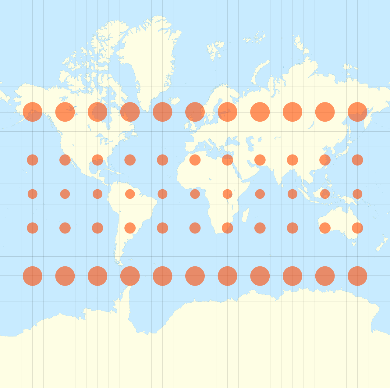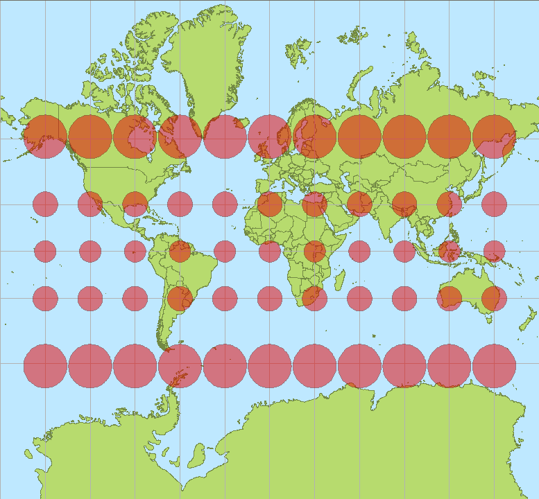| | 1569 | [Mercator](https://en.wikipedia.org/wiki/Mercator_projection "Mercator projection") <br>= Wright | [](https://en.wikipedia.org/wiki/File:Mercator_projection_Square.JPG) | Cylindrical | Conformal | [Gerardus Mercator](https://en.wikipedia.org/wiki/Gerardus_Mercator "Gerardus Mercator") | Lines of constant bearing (rhumb lines) are straight, aiding navigation. Areas inflate with latitude, becoming so extreme that the map cannot show the poles. 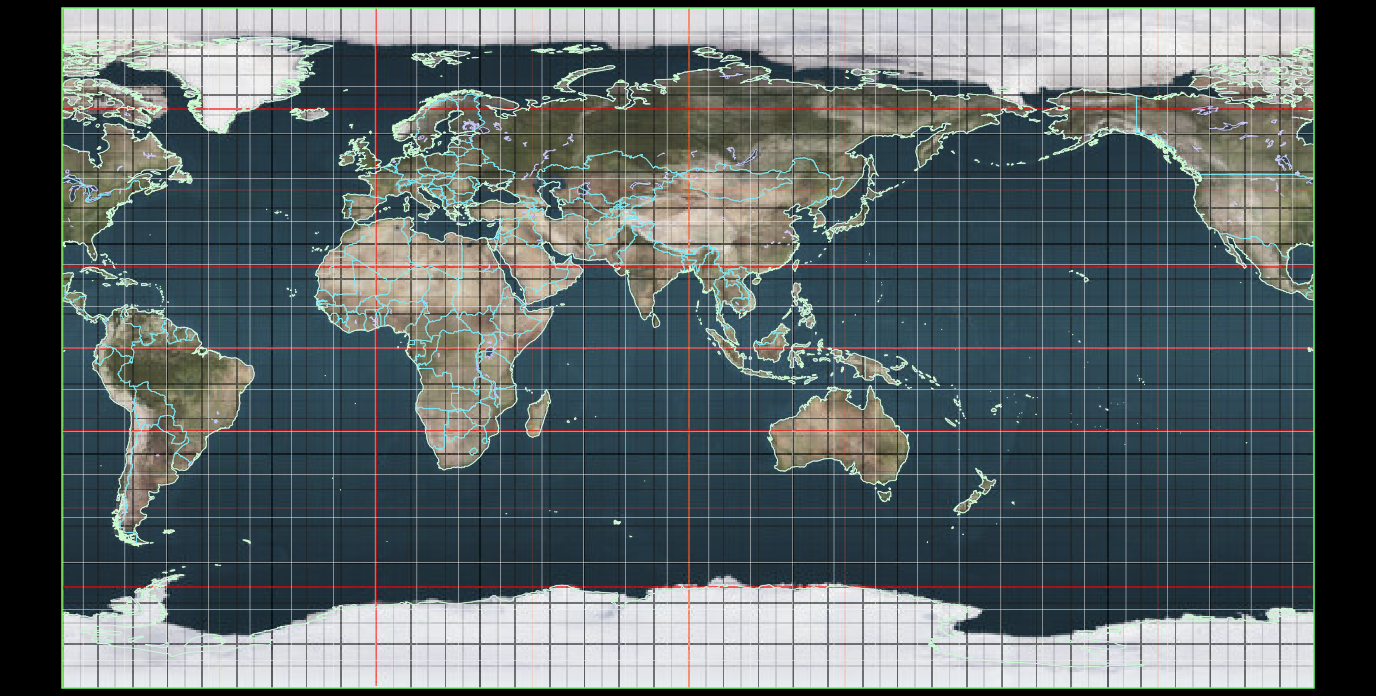| | 2005 | [Web Mercator](https://en.wikipedia.org/wiki/Web_Mercator "Web Mercator")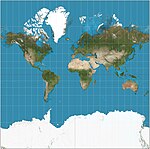 | [](https://en.wikipedia.org/wiki/File:Web_maps_Mercator_projection_SW.jpg) | Cylindrical | Compromise | [Google](https://en.wikipedia.org/wiki/Google "Google") | Variant of [Mercator](https://en.wikipedia.org/wiki/Mercator_projection "Mercator projection") that ignores Earth's ellipticity for fast calculation, and clips latitudes to ~85.05° for square presentation. De facto standard for Web mapping applications. | | 1822 | [Gauss–Krüger](https://en.wikipedia.org/wiki/Transverse_Mercator_projection#Ellipsoidal_transverse_Mercator "Transverse Mercator projection") <br>= Gauss conformal <br>= (ellipsoidal) transverse Mercator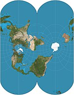 | [](https://en.wikipedia.org/wiki/File:Ellipsoidal_transverse_Mercator_projection_SW.jpg) | Cylindrical | Conformal | [Carl Friedrich Gauss](https://en.wikipedia.org/wiki/Carl_Friedrich_Gauss "Carl Friedrich Gauss")<br><br>[Johann Heinrich Louis Krüger](https://en.wikipedia.org/wiki/Johann_Heinrich_Louis_Kr%C3%BCger "Johann Heinrich Louis Krüger") | This transverse, ellipsoidal form of the Mercator is finite, unlike the equatorial Mercator. Forms the basis of the [Universal Transverse Mercator coordinate system](https://en.wikipedia.org/wiki/Universal_Transverse_Mercator_coordinate_system "Universal Transverse Mercator coordinate system"). | | 1922 | [Roussilhe oblique stereographic](https://en.wikipedia.org/wiki/Roussilhe_oblique_stereographic_projection "Roussilhe oblique stereographic projection") | | | | Henri Roussilhe | | | 1903 | Hotine oblique Mercator | [](https://en.wikipedia.org/wiki/File:Hotine_Mercator_projection_SW.jpg) | Cylindrical | Conformal | M. Rosenmund, J. Laborde, Martin Hotine | | | 1855 | [Gall stereographic](https://en.wikipedia.org/wiki/Gall_stereographic_projection "Gall stereographic projection")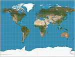 | [](https://en.wikipedia.org/wiki/File:Gall_Stereographic_projection_SW_centered.jpg) | Cylindrical | Compromise | [James Gall](https://en.wikipedia.org/wiki/James_Gall "James Gall") | Intended to resemble the Mercator while also displaying the poles. Standard parallels at 45°N/S. | | 1942 | [Miller](https://en.wikipedia.org/wiki/Miller_projection "Miller projection") <br>= Miller cylindrical | [](https://en.wikipedia.org/wiki/File:Miller_projection_SW.jpg) | Cylindrical | Compromise | [Osborn Maitland Miller](https://en.wikipedia.org/wiki/Osborn_Maitland_Miller "Osborn Maitland Miller") | Intended to resemble the Mercator while also displaying the poles. 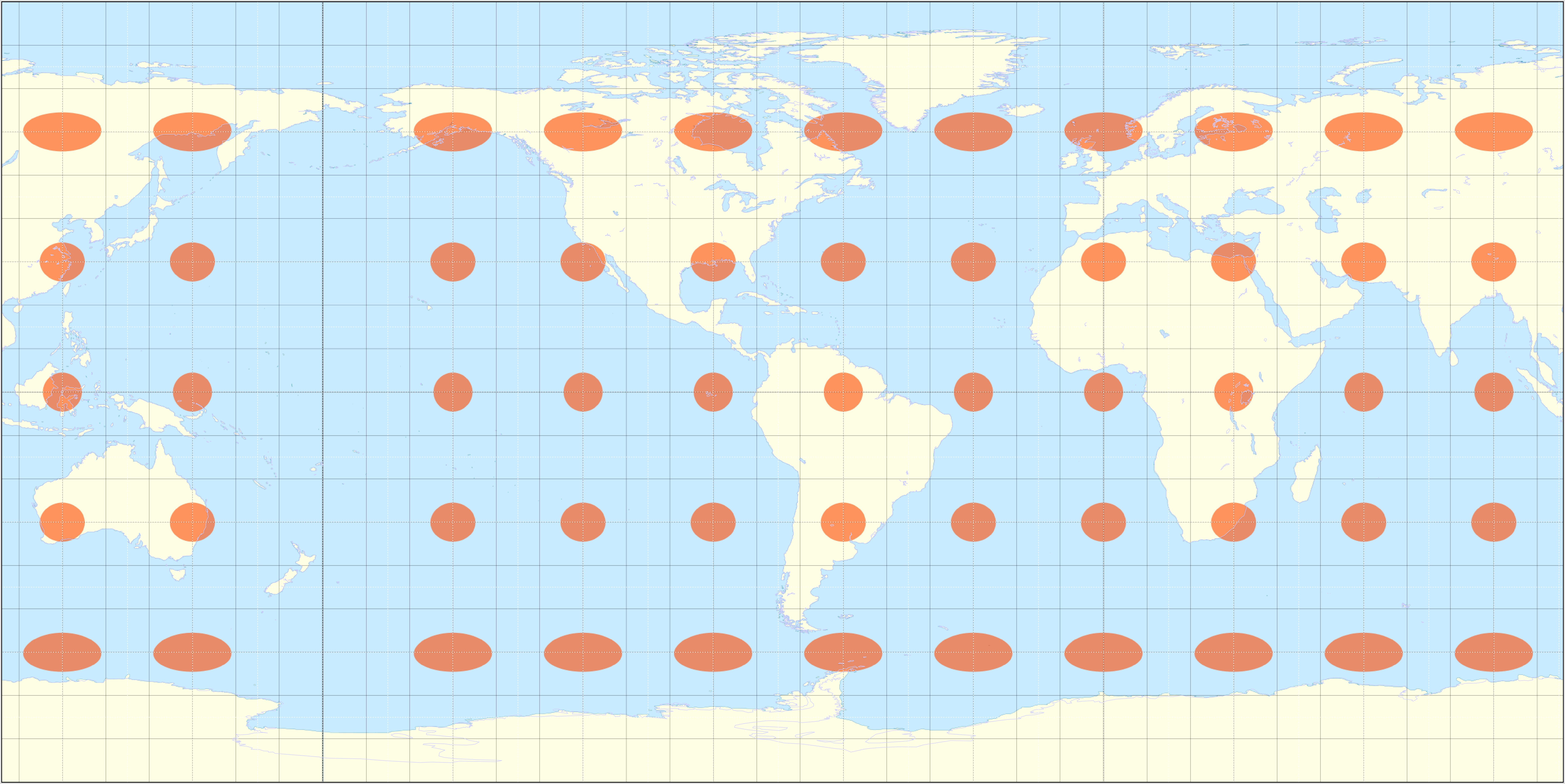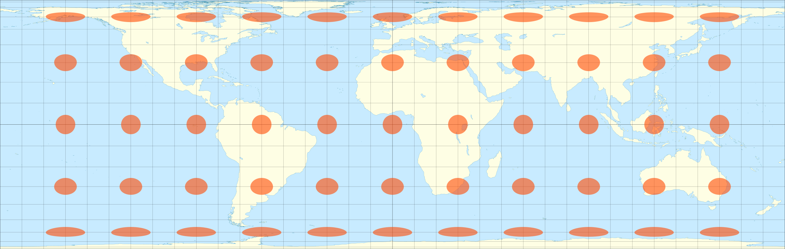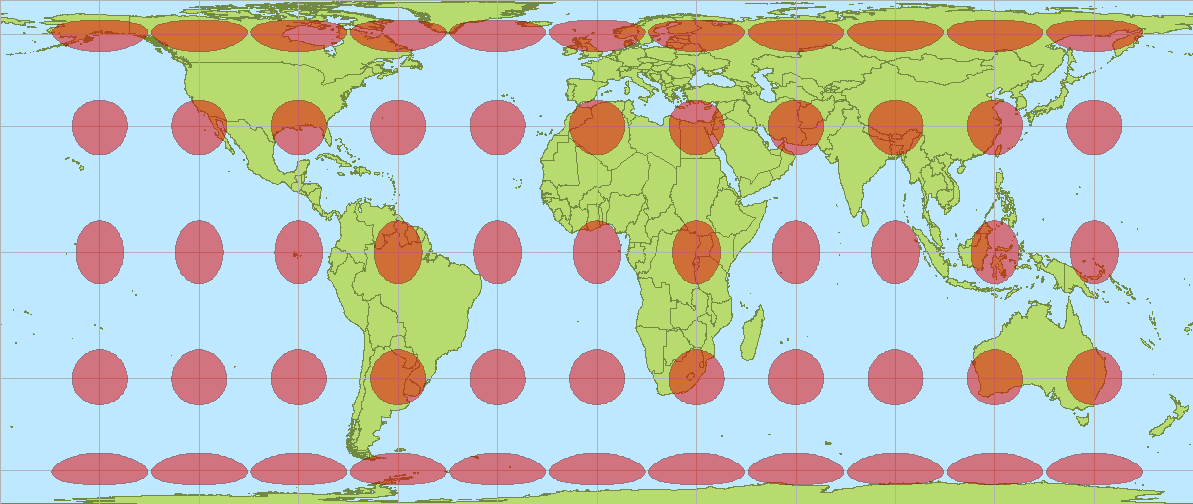| | 1772 | [Lambert cylindrical equal-area](https://en.wikipedia.org/wiki/Lambert_cylindrical_equal-area_projection "Lambert cylindrical equal-area projection") | [](https://en.wikipedia.org/wiki/File:Lambert_cylindrical_equal-area_projection_SW.jpg) | Cylindrical | Equal-area | [Johann Heinrich Lambert](https://en.wikipedia.org/wiki/Johann_Heinrich_Lambert "Johann Heinrich Lambert") | [Cylindrical equal-area projection](https://en.wikipedia.org/wiki/Cylindrical_equal-area_projection "Cylindrical equal-area projection") with standard parallel at the equator and an aspect ratio of π (3.14). 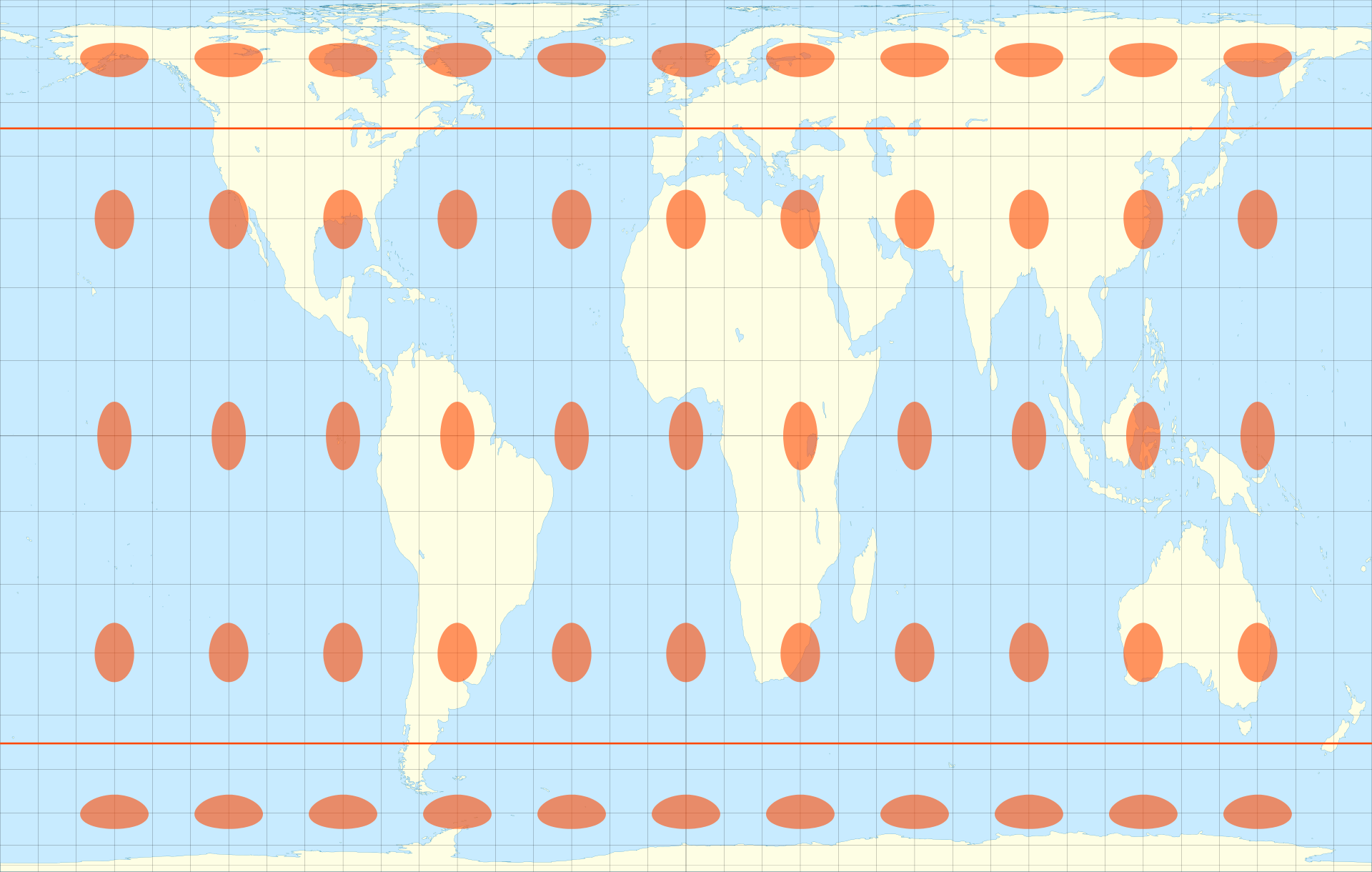| | 1910 | [Behrmann](https://en.wikipedia.org/wiki/Behrmann_projection "Behrmann projection") | [](https://en.wikipedia.org/wiki/File:Behrmann_projection_SW.jpg) | Cylindrical | Equal-area | [Walter Behrmann](https://en.wikipedia.org/wiki/Walter_Behrmann "Walter Behrmann") | [Cylindrical equal-area projection](https://en.wikipedia.org/wiki/Cylindrical_equal-area_projection "Cylindrical equal-area projection") with standard parallels at 30°N/S and an aspect ratio of (3/4)π ≈ 2.356. 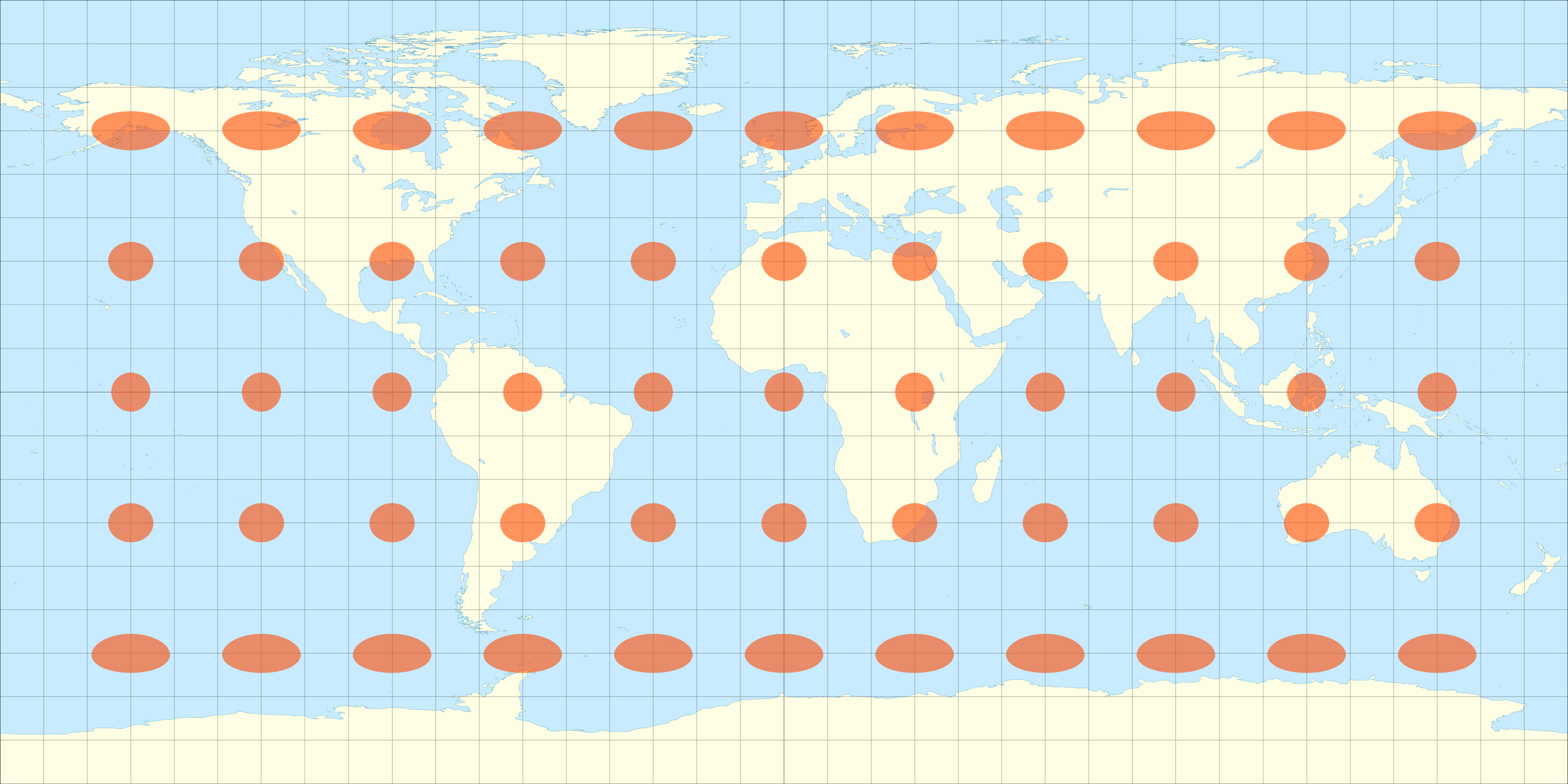| | 2002 | [Hobo–Dyer](https://en.wikipedia.org/wiki/Hobo%E2%80%93Dyer_projection "Hobo–Dyer projection") | [](https://en.wikipedia.org/wiki/File:Hobo%E2%80%93Dyer_projection_SW.jpg) | Cylindrical | Equal-area | | [Cylindrical equal-area projection](https://en.wikipedia.org/wiki/Cylindrical_equal-area_projection "Cylindrical equal-area projection") with standard parallels at 37.5°N/S and an aspect ratio of 1.977. Similar are Trystan Edwards with standard parallels at 37.4° and Smyth equal surface (=Craster rectangular) with standard parallels around 37.07°. | | 1855 | [Gall–Peters](https://en.wikipedia.org/wiki/Gall%E2%80%93Peters_projection "Gall–Peters projection") <br>= Gall orthographic <br>= Peters | [](https://en.wikipedia.org/wiki/File:Gall%E2%80%93Peters_projection_SW.jpg) | Cylindrical | Equal-area | [James Gall](https://en.wikipedia.org/wiki/James_Gall "James Gall")<br><br>([Arno Peters](https://en.wikipedia.org/wiki/Arno_Peters "Arno Peters")) | [Cylindrical equal-area projection](https://en.wikipedia.org/wiki/Cylindrical_equal-area_projection "Cylindrical equal-area projection") with standard parallels at 45°N/S and an aspect ratio of π/2 ≈ 1.571. Similar is Balthasart with standard parallels at 50°N/S and Tobler’s world in a square with standard parallels around 55.66°N/S. | | c. 1850 | [Central cylindrical](https://en.wikipedia.org/wiki/Central_cylindrical_projection "Central cylindrical projection") | [](https://en.wikipedia.org/wiki/File:Central_cylindric_projection_square.JPG) | Cylindrical | Perspective | (unknown) | Practically unused in cartography because of severe polar distortion, but popular in [panoramic photography](https://en.wikipedia.org/wiki/Panoramic_photography "Panoramic photography"), especially for architectural scenes. 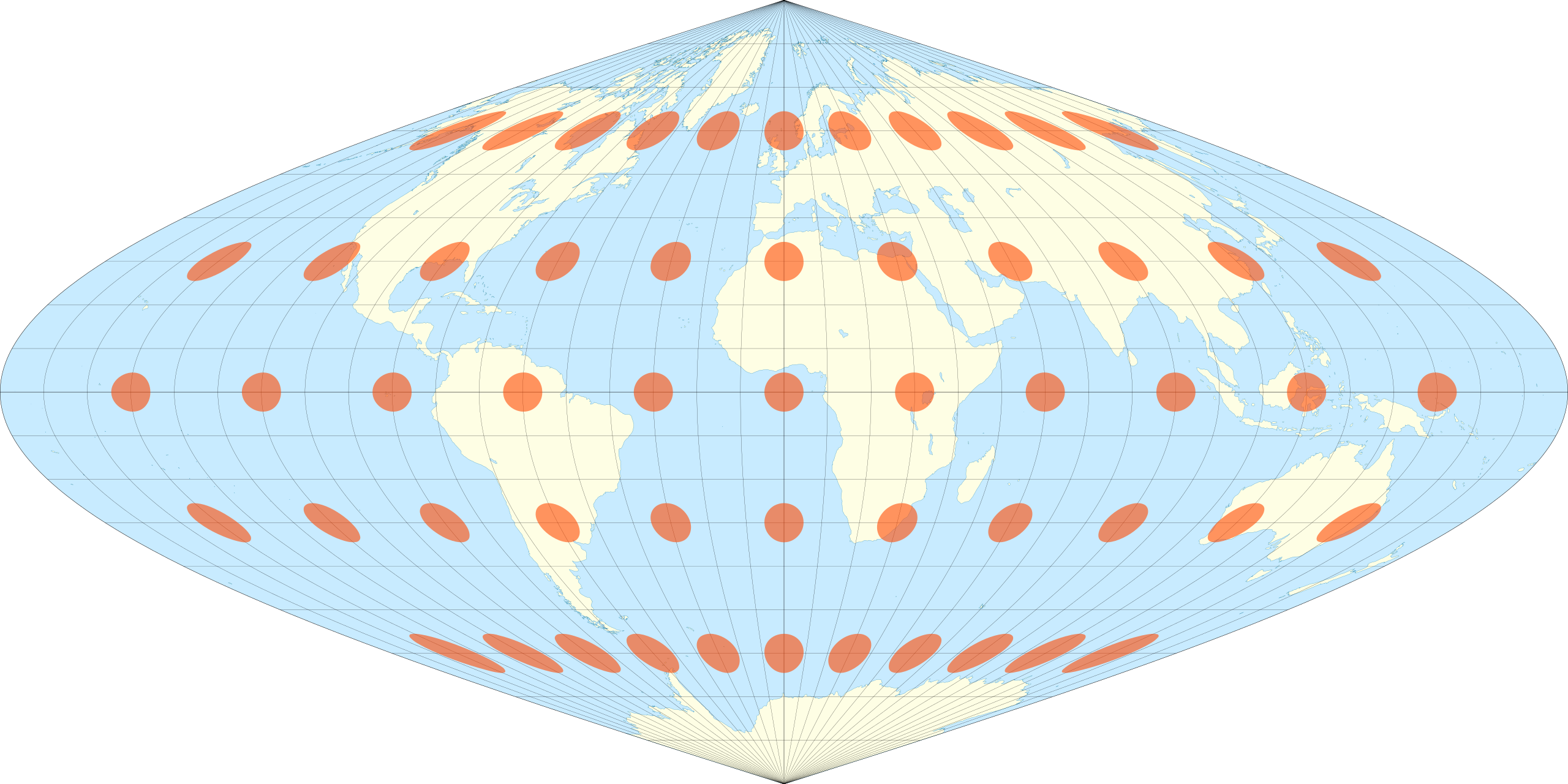| | c. 1600 | [Sinusoidal](https://en.wikipedia.org/wiki/Sinusoidal_projection "Sinusoidal projection") <br>= Sanson–Flamsteed <br>= Mercator equal-area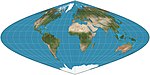 | [](https://en.wikipedia.org/wiki/File:Sinusoidal_projection_SW.jpg) | Pseudocylindrical | Equal-area, equidistant | (Several; first is unknown) | Meridians are sinusoids; parallels are equally spaced. Aspect ratio of 2:1. Distances along parallels are conserved. | | 1805 | [Mollweide](https://en.wikipedia.org/wiki/Mollweide_projection "Mollweide projection") <br>= elliptical <br>= Babinet <br>= homolographic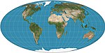 | [](https://en.wikipedia.org/wiki/File:Mollweide_projection_SW.jpg) | Pseudocylindrical | Equal-area | [Karl Brandan Mollweide](https://en.wikipedia.org/wiki/Karl_Brandan_Mollweide "Karl Brandan Mollweide") | Meridians are ellipses. | | 1906 | [Eckert II](https://en.wikipedia.org/wiki/Eckert_II_projection "Eckert II projection") | [](https://en.wikipedia.org/wiki/File:Eckert_II_projection_SW.JPG) | Pseudocylindrical | Equal-area | [Max Eckert-Greifendorff](https://en.wikipedia.org/wiki/Max_Eckert-Greifendorff "Max Eckert-Greifendorff") | | | 1906 | [Eckert IV](https://en.wikipedia.org/wiki/Eckert_IV_projection "Eckert IV projection")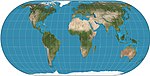 | [](https://en.wikipedia.org/wiki/File:Ecker_IV_projection_SW.jpg) | Pseudocylindrical | Equal-area | [Max Eckert-Greifendorff](https://en.wikipedia.org/wiki/Max_Eckert-Greifendorff "Max Eckert-Greifendorff") | Parallels are unequal in spacing and scale; outer meridians are semicircles; other meridians are semiellipses. | | 1906 | [Eckert VI](https://en.wikipedia.org/wiki/Eckert_VI_projection "Eckert VI projection") | [](https://en.wikipedia.org/wiki/File:Ecker_VI_projection_SW.jpg) | Pseudocylindrical | Equal-area | [Max Eckert-Greifendorff](https://en.wikipedia.org/wiki/Max_Eckert-Greifendorff "Max Eckert-Greifendorff") | Parallels are unequal in spacing and scale; meridians are half-period sinusoids. | | 1540 | [Ortelius oval](https://en.wikipedia.org/wiki/Ortelius_oval_projection "Ortelius oval projection") | [](https://en.wikipedia.org/wiki/File:Ortelius_oval_projection_SW.JPG) | Pseudocylindrical | Compromise | [Battista Agnese](https://en.wikipedia.org/wiki/Battista_Agnese "Battista Agnese") | Meridians are circular.[[2]](https://en.wikipedia.org/wiki/List_of_map_projections#cite_note-2) | | 1923 | [Goode homolosine](https://en.wikipedia.org/wiki/Goode_homolosine_projection "Goode homolosine projection") | [](https://en.wikipedia.org/wiki/File:Goode_homolosine_projection_SW.jpg) | Pseudocylindrical | Equal-area | [John Paul Goode](https://en.wikipedia.org/wiki/John_Paul_Goode "John Paul Goode") | Hybrid of Sinusoidal and Mollweide projections. <br>Usually used in interrupted form. 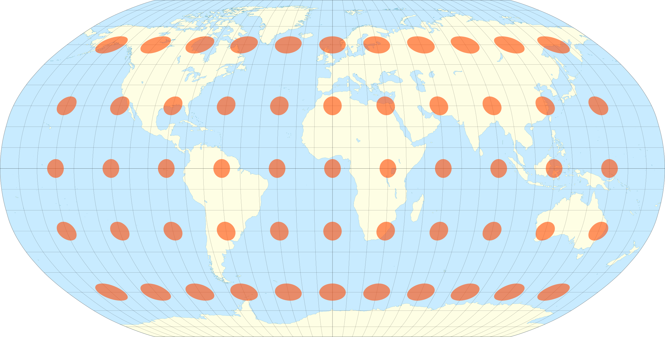| | 1939 | [Kavrayskiy VII](https://en.wikipedia.org/wiki/Kavrayskiy_VII_projection "Kavrayskiy VII projection") | [](https://en.wikipedia.org/wiki/File:Kavraiskiy_VII_projection_SW.jpg) | Pseudocylindrical | Compromise | [Vladimir V. Kavrayskiy](https://en.wikipedia.org/wiki/Vladimir_V._Kavrayskiy "Vladimir V. Kavrayskiy") | Evenly spaced parallels. Equivalent to Wagner VI horizontally compressed by a factor of 3/2. | | 1963 | [Robinson](https://en.wikipedia.org/wiki/Robinson_projection "Robinson projection")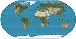 | [](https://en.wikipedia.org/wiki/File:Robinson_projection_SW.jpg) | Pseudocylindrical | Compromise | [Arthur H. Robinson](https://en.wikipedia.org/wiki/Arthur_H._Robinson "Arthur H. Robinson") | Computed by interpolation of tabulated values. Used by Rand McNally since inception and used by [NGS](https://en.wikipedia.org/wiki/National_Geographic_Society "National Geographic Society") in 1988–1998. | | 2018 | [Equal Earth](https://en.wikipedia.org/wiki/Equal_Earth_projection "Equal Earth projection") | [](https://en.wikipedia.org/wiki/File:Equal_Earth_projection_SW.jpg) | Pseudocylindrical | Equal-area | Bojan Šavrič, Tom Patterson, Bernhard Jenny | Inspired by the Robinson projection, but retains the relative size of areas. | | 2011 | [Natural Earth](https://en.wikipedia.org/wiki/Natural_Earth_projection "Natural Earth projection") | [](https://en.wikipedia.org/wiki/File:Natural_Earth_projection_SW.JPG) | Pseudocylindrical | Compromise | [Tom Patterson](https://en.wikipedia.org/w/index.php?title=Tom_Patterson_(cartographer)&action=edit&redlink=1 "Tom Patterson (cartographer) (page does not exist)") | Originally by interpolation of tabulated values. Now has a polynomial. | | 1973 | [Tobler hyperelliptical](https://en.wikipedia.org/wiki/Tobler_hyperelliptical_projection "Tobler hyperelliptical projection")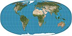 | [](https://en.wikipedia.org/wiki/File:Tobler_hyperelliptical_projection_SW.jpg) | Pseudocylindrical | Equal-area | [Waldo R. Tobler](https://en.wikipedia.org/wiki/Waldo_R._Tobler "Waldo R. Tobler") | A family of map projections that includes as special cases Mollweide projection, Collignon projection, and the various cylindrical equal-area projections. 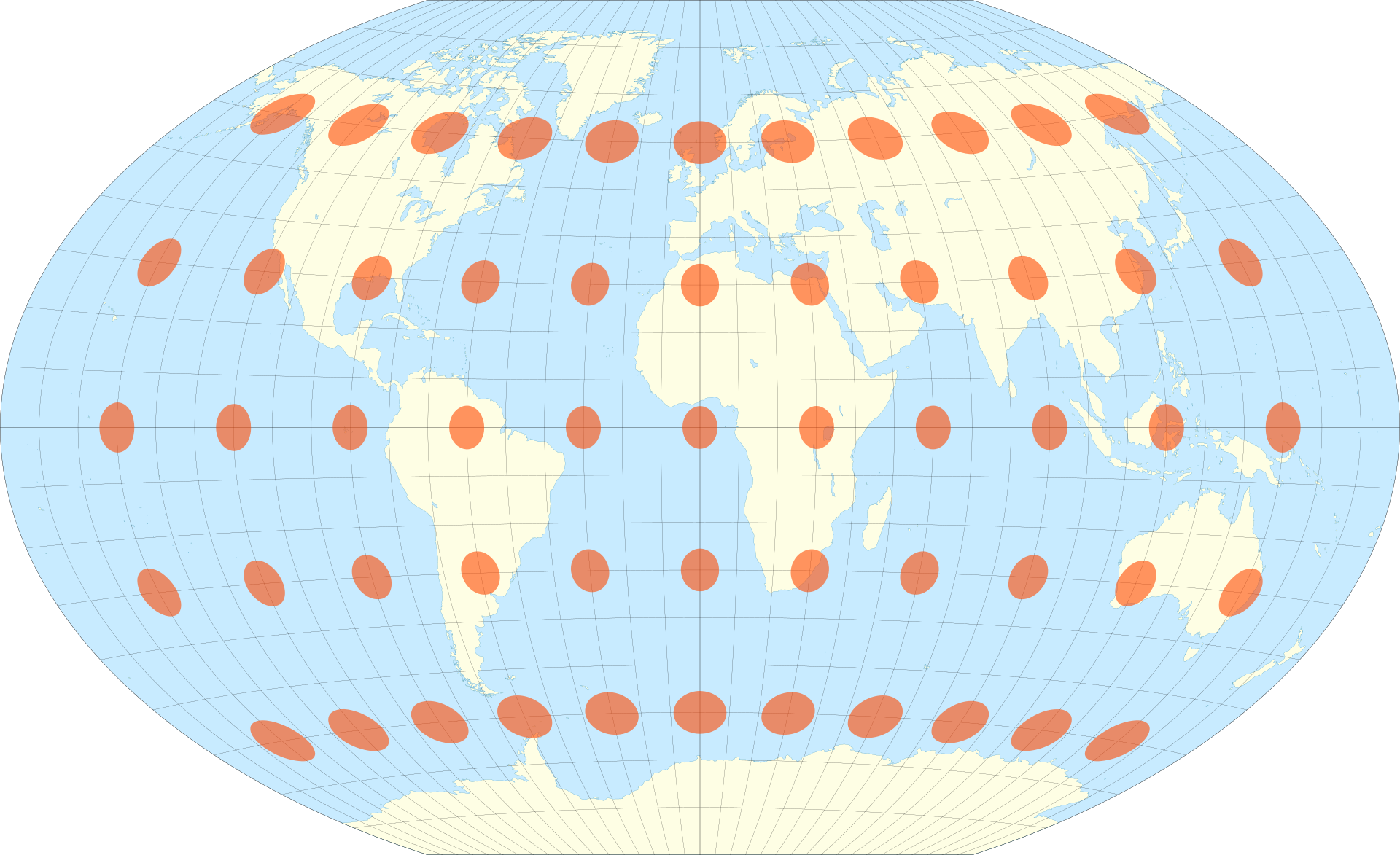| | 1932 | [Wagner VI](https://en.wikipedia.org/wiki/Wagner_VI_projection "Wagner VI projection")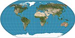 | [](https://en.wikipedia.org/wiki/File:Wagner_VI_projection_SW.jpg) | Pseudocylindrical | Compromise | [K. H. Wagner](https://en.wikipedia.org/w/index.php?title=K._H._Wagner&action=edit&redlink=1 "K. H. Wagner (page does not exist)") | Equivalent to Kavrayskiy VII vertically compressed by a factor of 3/2. | | c. 1865 | [Collignon](https://en.wikipedia.org/wiki/Collignon_projection "Collignon projection") | [](https://en.wikipedia.org/wiki/File:Collignon_projection_SW.jpg) | Pseudocylindrical | Equal-area | [Édouard Collignon](https://en.wikipedia.org/wiki/%C3%89douard_Collignon "Édouard Collignon") | Depending on configuration, the projection also may map the sphere to a single diamond or a pair of squares. | | 1997 | [HEALPix](https://en.wikipedia.org/wiki/HEALPix "HEALPix") | [](https://en.wikipedia.org/wiki/File:HEALPix_projection_SW.svg) | Pseudocylindrical | Equal-area | [Krzysztof M. Górski](https://en.wikipedia.org/w/index.php?title=Krzysztof_M._G%C3%B3rski&action=edit&redlink=1 "Krzysztof M. Górski (page does not exist)") | Hybrid of Collignon + Lambert cylindrical equal-area. | | 1929 | [Boggs eumorphic](https://en.wikipedia.org/wiki/Boggs_eumorphic_projection "Boggs eumorphic projection")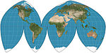 | [](https://en.wikipedia.org/wiki/File:Boggs_eumorphic_projection_SW.JPG) | Pseudocylindrical | Equal-area | Samuel Whittemore Boggs | The equal-area projection that results from average of sinusoidal and Mollweide _y_-coordinates and thereby constraining the _x_ coordinate. | | 1929 | Craster parabolic <br>=Putniņš P4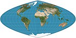 | [](https://en.wikipedia.org/wiki/File:Craster_parabolic_projection_SW.jpg) | Pseudocylindrical | Equal-area | John Craster | Meridians are parabolas. Standard parallels at 36°46′N/S; parallels are unequal in spacing and scale; 2:1 aspect. | | 1949 | McBryde–Thomas flat-pole quartic <br>= McBryde–Thomas #4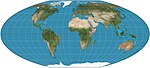 | [](https://en.wikipedia.org/wiki/File:McBryde-Thomas_flat-pole_quartic_projection_SW.jpg) | Pseudocylindrical | Equal-area | Felix W. McBryde, Paul Thomas | Standard parallels at 33°45′N/S; parallels are unequal in spacing and scale; meridians are fourth-order curves. Distortion-free only where the standard parallels intersect the central meridian. | | 1937<br><br>1944 | [Quartic authalic](https://en.wikipedia.org/wiki/Quartic_authalic "Quartic authalic")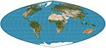 | [](https://en.wikipedia.org/wiki/File:Quartic_authalic_projection_SW.jpg) | Pseudocylindrical | Equal-area | Karl Siemon<br><br>Oscar Adams | Parallels are unequal in spacing and scale. No distortion along the equator. Meridians are fourth-order curves. | | 1965 | The Times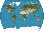 | [](https://en.wikipedia.org/wiki/File:The_Times_projection_SW.jpg) | Pseudocylindrical | Compromise | John Muir | Standard parallels 45°N/S. Parallels based on Gall stereographic, but with curved meridians. Developed for Bartholomew Ltd., The Times Atlas. | | 1935<br><br>1966 | [Loximuthal](https://en.wikipedia.org/wiki/Loximuthal_projection "Loximuthal projection")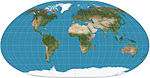 | [](https://en.wikipedia.org/wiki/File:Loximuthal_projection_SW.JPG) | Pseudocylindrical | Compromise | Karl Siemon<br><br>[Waldo R. Tobler](https://en.wikipedia.org/wiki/Waldo_R._Tobler "Waldo R. Tobler") | From the designated centre, lines of constant bearing (rhumb lines/loxodromes) are straight and have the correct length. Generally asymmetric about the equator. | | 1889 | [Aitoff](https://en.wikipedia.org/wiki/Aitoff_projection "Aitoff projection")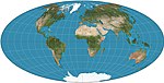 | [](https://en.wikipedia.org/wiki/File:Aitoff_projection_SW.jpg) | Pseudoazimuthal | Compromise | [David A. Aitoff](https://en.wikipedia.org/w/index.php?title=David_A._Aitoff&action=edit&redlink=1 "David A. Aitoff (page does not exist)") | Stretching of modified equatorial azimuthal equidistant map. Boundary is 2:1 ellipse. Largely superseded by Hammer. | | 1892 | [Hammer](https://en.wikipedia.org/wiki/Hammer_projection "Hammer projection") <br>= Hammer–Aitoff <br>variations: Briesemeister; Nordic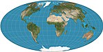 | [](https://en.wikipedia.org/wiki/File:Hammer_projection_SW.jpg) | Pseudoazimuthal | Equal-area | [Ernst Hammer](https://en.wikipedia.org/w/index.php?title=Ernst_Hammer_(cartographer)&action=edit&redlink=1 "Ernst Hammer (cartographer) (page does not exist)") | Modified from azimuthal equal-area equatorial map. Boundary is 2:1 ellipse. Variants are oblique versions, centred on 45°N. | | 1994 | [Strebe 1995](https://en.wikipedia.org/wiki/Strebe_1995_projection "Strebe 1995 projection")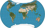 | [](https://en.wikipedia.org/wiki/File:Strebe_1995_11E_SW.jpg) | Pseudoazimuthal | Equal-area | Daniel "daan" Strebe | Formulated by using other equal-area map projections as transformations. | | 1921 | [Winkel tripel](https://en.wikipedia.org/wiki/Winkel_tripel_projection "Winkel tripel projection") | [](https://en.wikipedia.org/wiki/File:Winkel_triple_projection_SW.jpg) | Pseudoazimuthal | Compromise | [Oswald Winkel](https://en.wikipedia.org/wiki/Oswald_Winkel "Oswald Winkel") | Arithmetic mean of the [equirectangular projection](https://en.wikipedia.org/wiki/Equirectangular_projection "Equirectangular projection") and the [Aitoff projection](https://en.wikipedia.org/wiki/Aitoff_projection "Aitoff projection"). Standard world projection for the [NGS](https://en.wikipedia.org/wiki/National_Geographic_Society "National Geographic Society") since 1998. | | 1904 | [Van der Grinten](https://en.wikipedia.org/wiki/Van_der_Grinten_projection "Van der Grinten projection") | [](https://en.wikipedia.org/wiki/File:Van_der_Grinten_projection_SW.jpg) | Other | Compromise | [Alphons J. van der Grinten](https://en.wikipedia.org/w/index.php?title=Alphons_J._van_der_Grinten&action=edit&redlink=1 "Alphons J. van der Grinten (page does not exist)") | Boundary is a circle. All parallels and meridians are circular arcs. Usually clipped near 80°N/S. Standard world projection of the [NGS](https://en.wikipedia.org/wiki/National_Geographic_Society "National Geographic Society") in 1922–1988. | | c. 150 | [Equidistant conic](https://en.wikipedia.org/wiki/Equidistant_conic_projection "Equidistant conic projection") <br>= simple conic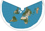 | [](https://en.wikipedia.org/wiki/File:Equidistant_conic_projection_SW.JPG) | Conic | Equidistant | Based on [Ptolemy](https://en.wikipedia.org/wiki/Ptolemy "Ptolemy")'s 1st Projection | Distances along meridians are conserved, as is distance along one or two standard parallels.[[3]](https://en.wikipedia.org/wiki/List_of_map_projections#cite_note-3) | | 1772 | [Lambert conformal conic](https://en.wikipedia.org/wiki/Lambert_conformal_conic_projection "Lambert conformal conic projection")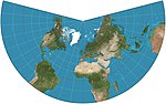 | [](https://en.wikipedia.org/wiki/File:Lambert_conformal_conic_projection_SW.jpg) | Conic | Conformal | [Johann Heinrich Lambert](https://en.wikipedia.org/wiki/Johann_Heinrich_Lambert "Johann Heinrich Lambert") | Used in aviation charts. | | 1805 | [Albers conic](https://en.wikipedia.org/wiki/Albers_conic_projection "Albers conic projection")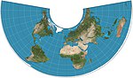 | [](https://en.wikipedia.org/wiki/File:Albers_projection_SW.jpg) | Conic | Equal-area | [Heinrich C. Albers](https://en.wikipedia.org/w/index.php?title=Heinrich_C._Albers&action=edit&redlink=1 "Heinrich C. Albers (page does not exist)") | Two standard parallels with low distortion between them. | | c. 1500 | [Werner](https://en.wikipedia.org/wiki/Werner_projection "Werner projection")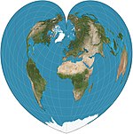 | [](https://en.wikipedia.org/wiki/File:Werner_projection_SW.jpg) | Pseudoconical | Equal-area, equidistant | [Johannes Stabius](https://en.wikipedia.org/wiki/Johannes_Stabius "Johannes Stabius") | Parallels are equally spaced concentric circular arcs. Distances from the [North Pole](https://en.wikipedia.org/wiki/North_Pole "North Pole") are correct as are the curved distances along parallels and distances along central meridian. | | 1511 | [Bonne](https://en.wikipedia.org/wiki/Bonne_projection "Bonne projection")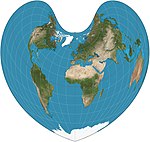 | [](https://en.wikipedia.org/wiki/File:Bonne_projection_SW.jpg) | Pseudoconical, cordiform | Equal-area, equidistant | [Bernardus Sylvanus](https://en.wikipedia.org/w/index.php?title=Bernardus_Sylvanus&action=edit&redlink=1 "Bernardus Sylvanus (page does not exist)") | Parallels are equally spaced concentric circular arcs and standard lines. Appearance depends on reference parallel. General case of both Werner and sinusoidal. | | 2003 | [Bottomley](https://en.wikipedia.org/wiki/Bottomley_projection "Bottomley projection")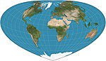 | [](https://en.wikipedia.org/wiki/File:Bottomley_projection_SW.JPG) | Pseudoconical | Equal-area | [Henry Bottomley](https://en.wikipedia.org/w/index.php?title=Henry_Bottomley&action=edit&redlink=1 "Henry Bottomley (page does not exist)") | Alternative to the Bonne projection with simpler overall shape <br><br>Parallels are elliptical arcs <br>Appearance depends on reference parallel. | | c. 1820 | [American polyconic](https://en.wikipedia.org/wiki/Polyconic_projection "Polyconic projection")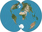 | [](https://en.wikipedia.org/wiki/File:American_Polyconic_projection.jpg) | Pseudoconical | Compromise | [Ferdinand Rudolph Hassler](https://en.wikipedia.org/wiki/Ferdinand_Rudolph_Hassler "Ferdinand Rudolph Hassler") | Distances along the parallels are preserved as are distances along the central meridian. | | c. 1853 | [Rectangular polyconic](https://en.wikipedia.org/wiki/Rectangular_polyconic_projection "Rectangular polyconic projection") | [](https://en.wikipedia.org/wiki/File:Rectangular_polyconic_projection_SW.jpg) | Pseudoconical | Compromise | [United States Coast Survey](https://en.wikipedia.org/wiki/United_States_Coast_and_Geodetic_Survey "United States Coast and Geodetic Survey") | Latitude along which scale is correct can be chosen. Parallels meet meridians at right angles. | | 1963 | [Latitudinally equal-differential polyconic](https://en.wikipedia.org/wiki/Latitudinally_equal-differential_polyconic_projection "Latitudinally equal-differential polyconic projection") | | Pseudoconical | Compromise | China State Bureau of Surveying and Mapping | Polyconic: parallels are non-concentric arcs of circles. | | c. 1000 | [Nicolosi globular](https://en.wikipedia.org/wiki/Nicolosi_globular_projection "Nicolosi globular projection")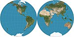 | [](https://en.wikipedia.org/wiki/File:Nicolosi_globular_projections_SW.jpg) | Pseudoconical[[4]](https://en.wikipedia.org/wiki/List_of_map_projections#cite_note-4) | Compromise | [Abū Rayḥān al-Bīrūnī](https://en.wikipedia.org/wiki/Al-Biruni "Al-Biruni"); reinvented by Giovanni Battista Nicolosi, 1660.[[1]](https://en.wikipedia.org/wiki/List_of_map_projections#cite_note-SnyderFlattening-1): 14 | | | 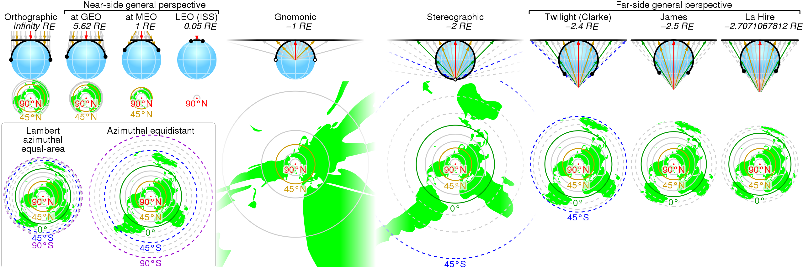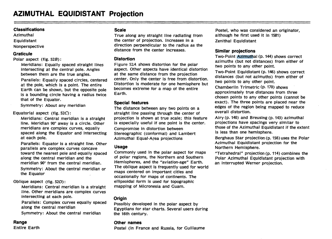c. 1000 | [Azimuthal equidistant](https://en.wikipedia.org/wiki/Azimuthal_equidistant_projection "Azimuthal equidistant projection") <br>=Postel <br>=zenithal equidistant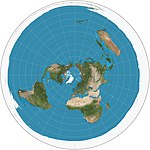 | [](https://en.wikipedia.org/wiki/File:Azimuthal_equidistant_projection_SW.jpg) | Azimuthal | Equidistant | [Abū Rayḥān al-Bīrūnī](https://en.wikipedia.org/wiki/Ab%C5%AB_Ray%E1%B8%A5%C4%81n_al-B%C4%ABr%C5%ABn%C4%AB "Abū Rayḥān al-Bīrūnī") | Distances from center are conserved. <br><br>Used as the [emblem](https://en.wikipedia.org/wiki/Flag_of_the_United_Nations "Flag of the United Nations") of the [United Nations](https://en.wikipedia.org/wiki/United_Nations "United Nations"), extending to 60° S. | | c. 580 BC | [Gnomonic](https://en.wikipedia.org/wiki/Gnomonic_projection "Gnomonic projection") | [](https://en.wikipedia.org/wiki/File:Gnomonic_projection_SW.jpg) | Azimuthal | Gnomonic | [Thales](https://en.wikipedia.org/wiki/Thales "Thales") (possibly) | All great circles map to straight lines. Extreme distortion far from the center. Shows less than one hemisphere. | | 1772 | [Lambert azimuthal equal-area](https://en.wikipedia.org/wiki/Lambert_azimuthal_equal-area_projection "Lambert azimuthal equal-area projection") | [](https://en.wikipedia.org/wiki/File:Lambert_azimuthal_equal-area_projection_SW.jpg) | Azimuthal | Equal-area | [Johann Heinrich Lambert](https://en.wikipedia.org/wiki/Johann_Heinrich_Lambert "Johann Heinrich Lambert") | The straight-line distance between the central point on the map to any other point is the same as the straight-line 3D distance through the globe between the two points. | | c. 200 BC | [Stereographic](https://en.wikipedia.org/wiki/Stereographic_map_projection "Stereographic map projection") | [](https://en.wikipedia.org/wiki/File:Stereographic_projection_SW.JPG) | Azimuthal | Conformal | [Hipparchos](https://en.wikipedia.org/wiki/Hipparchos "Hipparchos")* | Map is infinite in extent with outer hemisphere inflating severely, so it is often used as two hemispheres. Maps all small circles to circles, which is useful for planetary mapping to preserve the shapes of craters. | | c. 200 BC | [Orthographic](https://en.wikipedia.org/wiki/Orthographic_projection_in_cartography "Orthographic projection in cartography") | [](https://en.wikipedia.org/wiki/File:Orthographic_projection_SW.jpg) | Azimuthal | Perspective | [Hipparchos](https://en.wikipedia.org/wiki/Hipparchos "Hipparchos")* | View from an infinite distance. | | 1740 | [Vertical perspective](https://en.wikipedia.org/wiki/General_Perspective_projection "General Perspective projection") | [](https://en.wikipedia.org/wiki/File:Vertical_perspective_SW.jpg) | Azimuthal | Perspective | Matthias Seutter* | View from a finite distance. Can only display less than a hemisphere. | | 1919 | [Two-point equidistant](https://en.wikipedia.org/wiki/Two-point_equidistant_projection "Two-point equidistant projection")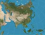 | [](https://en.wikipedia.org/wiki/File:Two-point_equidistant_projection_SW.jpg) | Azimuthal | Equidistant | Hans Maurer | Two "control points" can be almost arbitrarily chosen. The two straight-line distances from any point on the map to the two control points are correct. 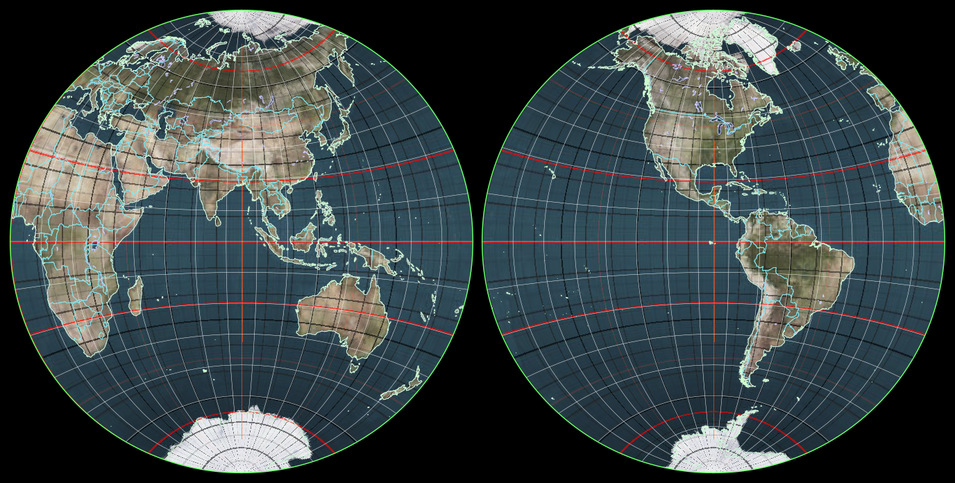| | 2021 | Gott, Goldberg and Vanderbei’s | [](https://en.wikipedia.org/wiki/File:Gott-Goldberg-Vanderbei_Projection.png) | Azimuthal | Equidistant | [J. Richard Gott](https://en.wikipedia.org/wiki/J._Richard_Gott "J. Richard Gott"), Goldberg and [Robert J. Vanderbei](https://en.wikipedia.org/wiki/Robert_J._Vanderbei "Robert J. Vanderbei") | Gott, Goldberg and Vanderbei’s double-sided disk map was designed to minimize all six types of map distortions. Not properly "a" map projection because it is on two surfaces instead of one, it consists of two hemispheric equidistant azimuthal projections back-to-back.[[5]](https://en.wikipedia.org/wiki/List_of_map_projections#cite_note-5)[[6]](https://en.wikipedia.org/wiki/List_of_map_projections#cite_note-6)[[7]](https://en.wikipedia.org/wiki/List_of_map_projections#cite_note-7) | | 1879 | [Peirce quincuncial](https://en.wikipedia.org/wiki/Peirce_quincuncial_projection "Peirce quincuncial projection") | [](https://en.wikipedia.org/wiki/File:Peirce_quincuncial_projection_SW.jpg) | Other | Conformal | [Charles Sanders Peirce](https://en.wikipedia.org/wiki/Charles_Sanders_Peirce "Charles Sanders Peirce") | Tessellates. Can be tiled continuously on a plane, with edge-crossings matching except for four singular points per tile. | | 1887 | [Guyou hemisphere-in-a-square projection](https://en.wikipedia.org/wiki/Guyou_hemisphere-in-a-square_projection "Guyou hemisphere-in-a-square projection")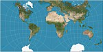 | [](https://en.wikipedia.org/wiki/File:Guyou_doubly_periodic_projection_SW.JPG) | Other | Conformal | [Émile Guyou](https://en.wikipedia.org/w/index.php?title=%C3%89mile_Guyou&action=edit&redlink=1 "Émile Guyou (page does not exist)") | Tessellates. | | 1925 | [Adams hemisphere-in-a-square projection](https://en.wikipedia.org/wiki/Adams_hemisphere-in-a-square_projection "Adams hemisphere-in-a-square projection") | [](https://en.wikipedia.org/wiki/File:Adams_hemisphere_in_a_square.JPG) | Other | Conformal | [Oscar Sherman Adams](https://en.wikipedia.org/w/index.php?title=Oscar_Sherman_Adams&action=edit&redlink=1 "Oscar Sherman Adams (page does not exist)") | | | 1965 | [Lee conformal world on a tetrahedron](https://en.wikipedia.org/wiki/Lee_Conformal_Projection "Lee Conformal Projection") | [](https://en.wikipedia.org/wiki/File:Lee_Conformal_World_in_a_Tetrahedron_projection.png) | Polyhedral | Conformal | [L. P. Lee](https://en.wikipedia.org/w/index.php?title=L._P._Lee&action=edit&redlink=1 "L. P. Lee (page does not exist)") | Projects the globe onto a regular tetrahedron. Tessellates. | | 1514 | [Octant projection](https://en.wikipedia.org/wiki/Octant_projection "Octant projection")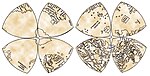 | [](https://en.wikipedia.org/wiki/File:Leonardo_da_Vinci%E2%80%99s_Mappamundi.jpg) | Polyhedral | Compromise | [Leonardo da Vinci](https://en.wikipedia.org/wiki/Leonardo_da_Vinci "Leonardo da Vinci") | Projects the globe onto eight octants ([Reuleaux triangles](https://en.wikipedia.org/wiki/Reuleaux_triangle "Reuleaux triangle")) with no meridians and no parallels. 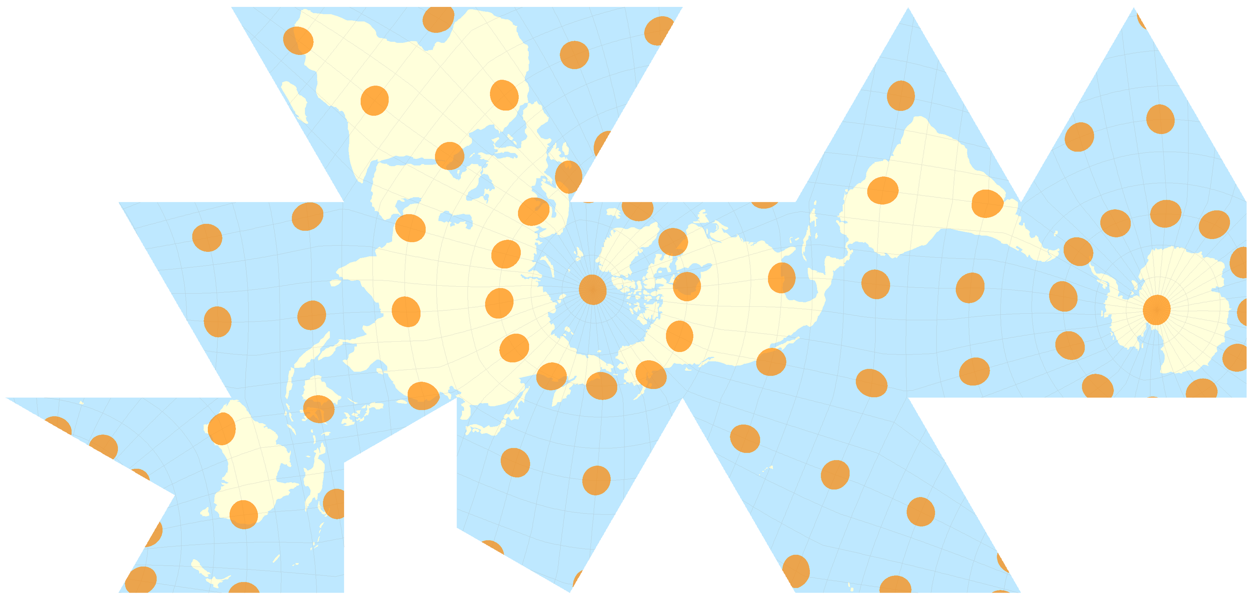| | 1909 | [Cahill's butterfly map](https://en.wikipedia.org/wiki/Cahill%27s_butterfly_map "Cahill's butterfly map") | [](https://en.wikipedia.org/wiki/File:Cahill_Butterfly_Map.jpg) | Polyhedral | Compromise | [Bernard Joseph Stanislaus Cahill](https://en.wikipedia.org/wiki/Bernard_J._S._Cahill "Bernard J. S. Cahill") | Projects the globe onto an octahedron with symmetrical components and contiguous landmasses that may be displayed in various arrangements. | | 1975 | [Cahill–Keyes projection](https://en.wikipedia.org/wiki/Cahill%E2%80%93Keyes_projection "Cahill–Keyes projection") | [](https://en.wikipedia.org/wiki/File:Cahill-Keyes_projection.png) | Polyhedral | Compromise | [Gene Keyes](https://en.wikipedia.org/wiki/Gene_Keyes "Gene Keyes") | Projects the globe onto a truncated octahedron with symmetrical components and contiguous land masses that may be displayed in various arrangements. | | 1996 | [Waterman butterfly projection](https://en.wikipedia.org/wiki/Waterman_butterfly_projection "Waterman butterfly projection")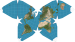 | [](https://en.wikipedia.org/wiki/File:Waterman_projection.png) | Polyhedral | Compromise | [Steve Waterman](https://en.wikipedia.org/w/index.php?title=Steve_Waterman_(mathematician)&action=edit&redlink=1 "Steve Waterman (mathematician) (page does not exist)") | Projects the globe onto a truncated octahedron with symmetrical components and contiguous land masses that may be displayed in various arrangements. | | 1973 | [Quadrilateralized spherical cube](https://en.wikipedia.org/wiki/Quadrilateralized_spherical_cube "Quadrilateralized spherical cube") | | Polyhedral | Equal-area | F. Kenneth Chan, E. M. O'Neill | | | 1943 | [Dymaxion map](https://en.wikipedia.org/wiki/Dymaxion_map "Dymaxion map") | [](https://en.wikipedia.org/wiki/File:Dymaxion_projection.png) | Polyhedral | Compromise | [Buckminster Fuller](https://en.wikipedia.org/wiki/Buckminster_Fuller "Buckminster Fuller") | Also known as a Fuller Projection. | | 1999 | [AuthaGraph projection](https://en.wikipedia.org/wiki/AuthaGraph_projection "AuthaGraph projection") | [](https://en.wikipedia.org/wiki/File:Projection_AuthaGraph.png) | Polyhedral | Compromise | [Hajime Narukawa](https://en.wikipedia.org/wiki/Hajime_Narukawa "Hajime Narukawa") | Approximately equal-area. Tessellates. | | 2008 | [Myriahedral projections](https://en.wikipedia.org/w/index.php?title=Myriahedral_projection&action=edit&redlink=1 "Myriahedral projection (page does not exist)") | | Polyhedral | Equal-area | [Jarke J. van Wijk](https://en.wikipedia.org/wiki/Jack_van_Wijk "Jack van Wijk") | Projects the globe onto a myriahedron: a polyhedron with a very large number of faces.[[8]](https://en.wikipedia.org/wiki/List_of_map_projections#cite_note-8)[[9]](https://en.wikipedia.org/wiki/List_of_map_projections#cite_note-9) | | 1909 | [Craig retroazimuthal](https://en.wikipedia.org/wiki/Craig_retroazimuthal_projection "Craig retroazimuthal projection") <br>= Mecca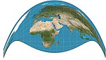 | [](https://en.wikipedia.org/wiki/File:Craig_projection_SW.jpg) | Retroazimuthal | Compromise | James Ireland Craig | | | 1910 | [Hammer retroazimuthal, front hemisphere](https://en.wikipedia.org/wiki/Hammer_retroazimuthal_projection "Hammer retroazimuthal projection")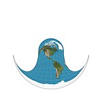 | [](https://en.wikipedia.org/wiki/File:Hammer_retroazimuthal_projection_front_SW.JPG) | Retroazimuthal | | [Ernst Hammer](https://en.wikipedia.org/w/index.php?title=Ernst_Hammer_(cartographer)&action=edit&redlink=1 "Ernst Hammer (cartographer) (page does not exist)") | | | 1910 | [Hammer retroazimuthal, back hemisphere](https://en.wikipedia.org/wiki/Hammer_retroazimuthal_projection "Hammer retroazimuthal projection") | [](https://en.wikipedia.org/wiki/File:Hammer_retroazimuthal_projection_back_SW.JPG) | Retroazimuthal | | [Ernst Hammer](https://en.wikipedia.org/w/index.php?title=Ernst_Hammer_(cartographer)&action=edit&redlink=1 "Ernst Hammer (cartographer) (page does not exist)") | | | 1833 | [Littrow](https://en.wikipedia.org/wiki/Littrow_projection "Littrow projection") | [](https://en.wikipedia.org/wiki/File:Littrow_projection_SW.JPG) | Retroazimuthal | Conformal | [Joseph Johann Littrow](https://en.wikipedia.org/wiki/Joseph_Johann_Littrow "Joseph Johann Littrow") | on equatorial aspect it shows a hemisphere except for poles. | | 1943 | [Armadillo](https://en.wikipedia.org/wiki/Armadillo_projection "Armadillo projection") | [](https://en.wikipedia.org/wiki/File:Armadillo_projection_SW.JPG) | Other | Compromise | [Erwin Raisz](https://en.wikipedia.org/wiki/Erwin_Raisz "Erwin Raisz") | | | 1982 | [GS50](https://en.wikipedia.org/wiki/GS50_projection "GS50 projection") | [](https://en.wikipedia.org/wiki/File:GS50_projection.png) | Other | Conformal | [John P. Snyder](https://en.wikipedia.org/wiki/John_P._Snyder "John P. Snyder") | Designed specifically to minimize distortion when used to display all 50 [U.S. states](https://en.wikipedia.org/wiki/U.S._state "U.S. state"). | | 1941 | Wagner VII <br>= Hammer-Wagner | [](https://en.wikipedia.org/wiki/File:Wagner-VII_world_map_projection.jpg) | Pseudoazimuthal | Equal-area | K. H. Wagner | | | 1947? | [Chamberlin trimetric projection](https://en.wikipedia.org/wiki/Chamberlin_trimetric_projection "Chamberlin trimetric projection") | [](https://en.wikipedia.org/wiki/File:Chamberlin_trimetric_projection_SW.jpg) | Other | Compromise | Wellman Chamberlin | Many National Geographic Society maps of single continents use this projection. | | 1948 | Atlantis <br>= Transverse Mollweide | [](https://en.wikipedia.org/wiki/File:Atlantis-landscape.jpg) | Pseudocylindrical | Equal-area | John Bartholomew | Oblique version of Mollweide | | 1953 | Bertin <br>= Bertin-Rivière <br>= Bertin 1953 | [](https://en.wikipedia.org/wiki/File:Bertin-map.jpg) | Other | Compromise | Jacques Bertin | Projection in which the compromise is no longer homogeneous but instead is modified for a larger deformation of the oceans, to achieve lesser deformation of the continents. Commonly used for French geopolitical maps.[[10]](https://en.wikipedia.org/wiki/List_of_map_projections#cite_note-10) | | 2002 | Hao projection | [](https://en.wikipedia.org/wiki/File:Hao_projection_(north).png) | Pseudoconical | Compromise | Hao Xiaoguang | Known as "plane terrestrial globe",[[11]](https://en.wikipedia.org/wiki/List_of_map_projections#cite_note-11) it was adopted by the [People's Liberation Army](https://en.wikipedia.org/wiki/People%27s_Liberation_Army "People's Liberation Army") for the official military maps and China’s State Oceanic Administration for polar expeditions.[[12]](https://en.wikipedia.org/wiki/List_of_map_projections#cite_note-12)[[13]](https://en.wikipedia.org/wiki/List_of_map_projections#cite_note-13) | *T ![[Attachments/Cylindrical.png]] ![[Attachments/Ae gridlines.png]] ![[Attachments/Mercaotor gridlines .png]] ![[Attachments/dual hemisphere.png]] ![[Attachments/gobualr .png]] ![[Attachments/mercator 2.png]] ![[Attachments/9 in noth 9 in south.png]] ![[Attachments/flgiht ae.pngwqwwq.png]] ![[Attachments/20 lines of lasde.png]] ![[Attachments/20 lines of lat.png]] ![[Attachments/wireframe.png]] ![[Attachments/photo_2024-02-24_16-07-03 2.jpg]] ![[Attachments/photo_2024-02-24_16-07-06 2.jpg]] ![[Attachments/photo_2024-02-24_16-07-09 2.jpg]] ![[Attachments/photo_2024-02-24_16-22-55 2.jpg]] ![[Attachments/photo_2024-02-24_16-24-00 2.png]] ![[Attachments/photo_2024-02-24_16-29-29 2.jpg]] ![[Attachments/robinson 2.jpg]] ![[Attachments/az mapped out 2.png]] ![[Attachments/rpboinsoon 2.jpg]] ![[Attachments/robinson mapped 2.png]] ![[Attachments/Los Angeles, CA—Zürich, Switzerland 2.png]] ![[Attachments/1920px-Tissot_indicatrix_world_map_Gall-Peters_equal-area_proj.svg 2.png]] ![[Attachments/2560px-Tissot_indicatrix_world_map_equirectangular_proj.svg 2.png]] ![[Attachments/Azimuthal_equidistant_projection_with_Tissot's_indicatrix 2.png]] ![[Attachments/Fuller_projection_with_Tissot's_indicatrix_of_deformation 2.png]] ![[Attachments/Stereographic_projection_with_Tissot's_indicatrix 2.png]] ![[Attachments/Tissot_indicatrix_world_map_Lambert_cyl_equal-area_proj.svg 2.png]] ![[Attachments/Tissot_indicatrix_world_map_Mercator_proj.svg 2.png]] ![[Attachments/Tissot_indicatrix_world_map_Mollweide_proj.svg 2.png]] ![[Attachments/Tissot_indicatrix_world_map_Robinson_proj.svg 2.png]] ![[Attachments/Tissot_indicatrix_world_map_sinusoidal_proj.svg 2.png]] ![[Attachments/Tissot_indicatrix_world_map_Winkel_Tripel_proj.svg 2.png]] ![[Attachments/Transverse_Mercator_projection_of_Standard_meridian_135E-45W_withTissot's_indicatrix 2.png]] ![[Attachments/robinson (2).jpg]] ![[Attachments/Tissot_behrmann 2.png]] ![[Attachments/Tissot_mercator 2.png]] ![[Attachments/photo_2024-02-24_16-24-00 (2).png]] ![[Attachments/photo_2024-02-24_16-29-29 (2).jpg]] ![[Attachments/photo_2024-02-24_16-07-00 2.jpg]] ![[Attachments/Map projections.pdf]]![[Attachments/Pasted image 20240414224720.png]] ![[Attachments/Pasted image 20240504040800.png]] 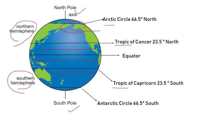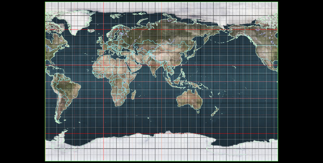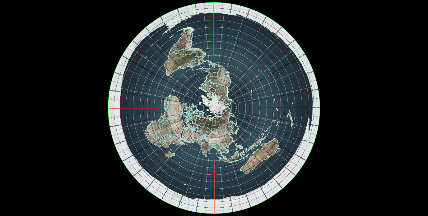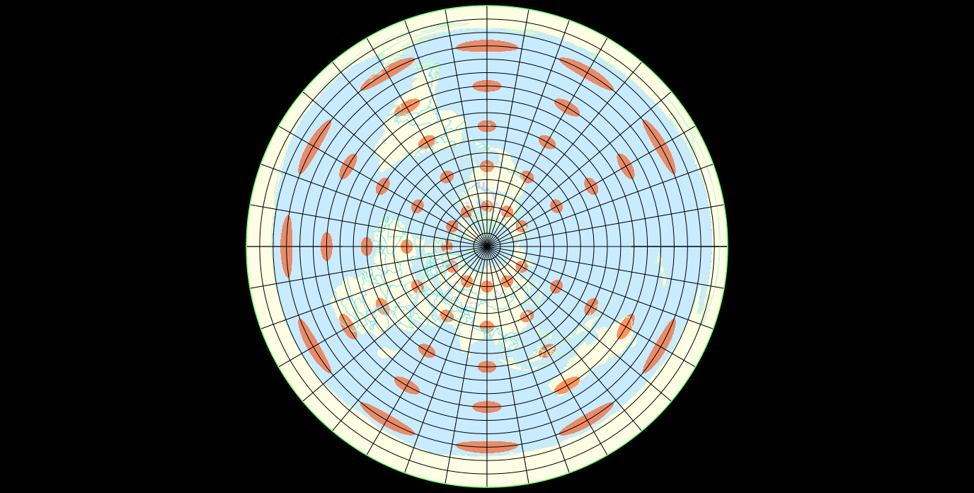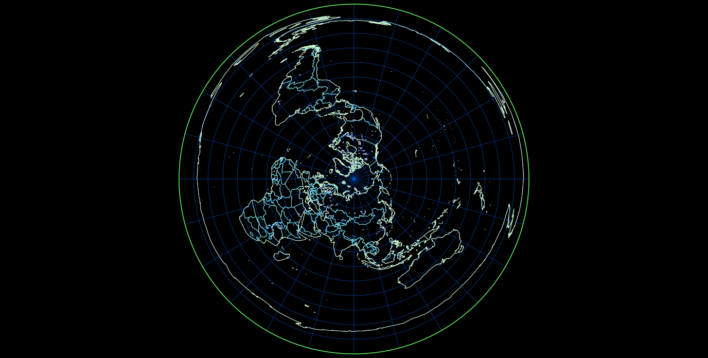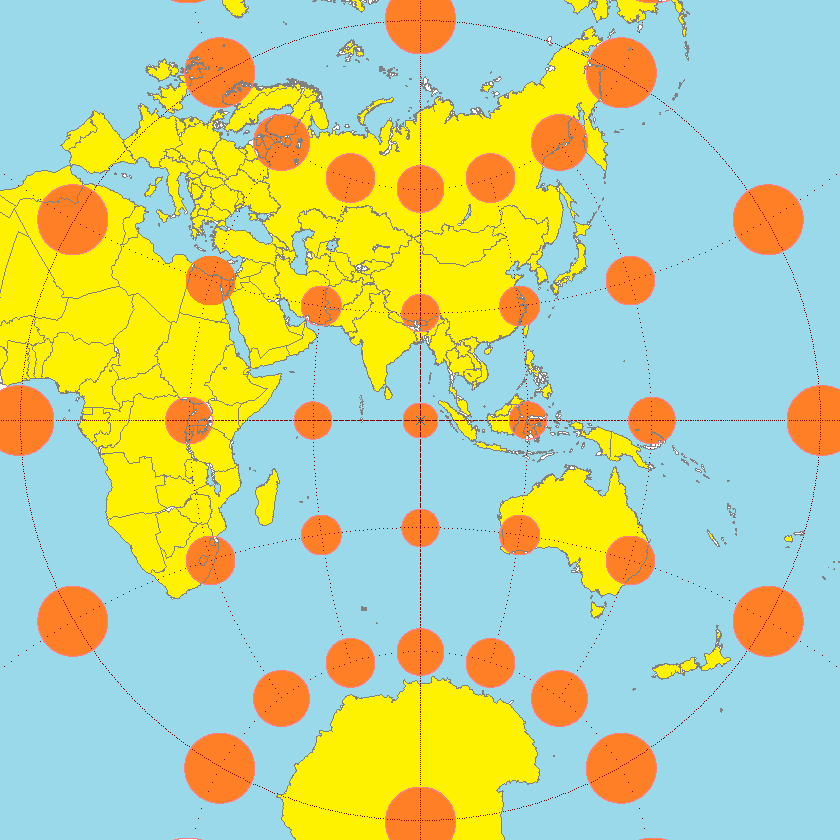Of course, since the Gleason map represents the exact same data as the globe, which is the same as every other map that uses the required longitude and latitude, the tropics are figured to be about 22,859 miles long. Because the math is based, of course, on the coordinate system....Its easy ### Geographical Measurements Using the Gleason Map: The Gleason map, like all maps using a longitude and latitude system, reflects measurements consistent with a single celestiaL SPHEREmodel. Using this model, the tropics' circumference is estimated based on their latitude. ### Basic Circumference Formula: For an approximate measurement, the formula for the circumference (𝑙l) of a circle at a given latitude (𝜙ϕ) on Earth is: 𝑙=2𝜋𝑅⋅cos⁡(𝜙)l=2πR⋅cos(ϕ) - 𝑅R is the Earth's mean radius, approximately 6,378.137 kilometers. - 𝜙ϕ is the latitude of interest in radians (e.g., the Tropic of Cancer). ### Adjusted Formula for Earth's Oblateness: To account for Earth's oblateness, an adjusted formula is used: 𝑙=2𝜋𝑅⋅cos⁡(𝜙)⋅(1−0.00669438sin⁡2(𝜙))−0.5l=2πR⋅cos(ϕ)⋅(1−0.00669438sin2(ϕ))−0.5 - This adjustment incorporates the eccentricity factor 0.006694380.00669438 and corrects for overestimation by adjusting the value slightly. ### Deriving Latitude from a Given Circumference: If you know the circumference (𝑙l) and want to find the corresponding latitude (𝜙ϕ), you use the inverse of the previous formula, rearranged to solve for 𝜙ϕ: 𝑙=2𝜋⋅cos⁡(𝜙)⋅6378137⋅(1−0.00669438sin⁡2(𝜙))−0.5l=2π⋅cos(ϕ)⋅6378137⋅(1−0.00669438sin2(ϕ))−0.5 Given 𝑙=36788l=36788 km, to find 𝜙ϕ, the equation: 36788=2𝜋⋅cos⁡(𝜙)⋅6378137⋅(1−0.00669438sin⁡2(𝜙))−0.536788=2π⋅cos(ϕ)⋅6378137⋅(1−0.00669438sin2(ϕ))−0.5 is used, where 𝜙ϕ must be calculated iteratively. ### Summary: These formulas help calculate the circumference at various latitudes, considering Earth's shape and ensuring precision in geographical measurements. The application of these formulas also extends to calculating latitudes based on known circumferences, essential for accurate global positioning and cartography. Circumference of tropics l=2πR⋅cos(ϕ) where R [radius of the Earth, approx 6378 kilometers] ϕ is the latitude of the Tropic of Cancer in radians. Or more accurately for your geoid..... l=2πR⋅cos(ϕ)⋅(1−0.00669438sin2(ϕ))−0.5 (I mean, we are better globers than you as well) Because YOU have to account for Earth's oblateness (flattening at the poles) using the eccentricity factor 0.006694380.00669438, and it subtracts 0.50.5 to adjust for possible overestimation. Of course, you can always go backwards, and derive the latitude at your current tropic by l = 2π cos(φ) ⋅ 6378137 ⋅ (1 - 0.00669438 sin^2(φ))^(-0.5) Given l = 36788 km, we can plug this value into the formula and solve for φ. 36788 = 2π cos(φ) ⋅ 6378137 ⋅ (1 - 0.00669438 sin^2(φ))^(-0.5) We have to denote φ = cos(φ) and φ = sin(φ), so our equation becomes: 36788 = 2φ ⋅ φ ⋅ 6378137 ⋅ (1 - 0.00669438 φ^2)^(-0.5 Right? And all we asked was the radius... 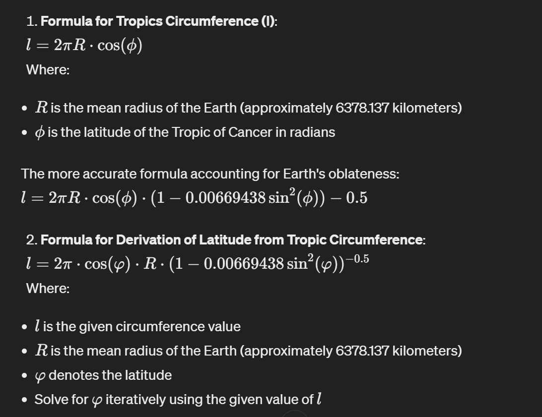![[Attachments/Pasted image 20240504040811.png]] ![[Attachments/Pasted image 20240504040819.png]] ### Formulas for Calculating the Circumference at a Specific Latitude #### 1. **Basic Formula for Tropics Circumference** The basic formula calculates the circumference at a specific latitude (𝜙ϕ): 𝑙=2𝜋𝑅⋅cos⁡(𝜙)l=2πR⋅cos(ϕ) - 𝑅R is the mean radius of the Earth, approximately 6378.137 kilometers. - 𝜙ϕ is the latitude, in radians, where you want to calculate the circumference. #### 2. **Adjusted Formula for Earth's Oblateness** This adjusted formula accounts for the Earth's oblateness, providing a more accurate circumference: 𝑙=2𝜋𝑅⋅cos⁡(𝜙)⋅(1−0.00669438sin⁡2(𝜙))−0.5l=2πR⋅cos(ϕ)⋅(1−0.00669438sin2(ϕ))−0.5 - The term 0.00669438sin⁡2(𝜙)0.00669438sin2(ϕ) adjusts for the elliptical shape of the Earth, which affects the actual radius at the given latitude. ### Procedure for Applying These Formulas: 1. **Convert Latitude to Radians**: If the latitude (𝜙ϕ) is provided in degrees, convert it to radians using the conversion radians=degrees×𝜋180radians=180degrees×π​. 2. **Apply the Basic or Adjusted Formula**: - Use the basic formula for approximate calculations or when high precision is not necessary. - Use the adjusted formula to incorporate Earth's oblateness for more precise calculations, especially relevant at extreme latitudes. ### Example: Calculating the Circumference of the Tropic of Cancer The Tropic of Cancer is located at approximately 23.43659 degrees north. To find the circumference along this latitude: 1. **Convert the Latitude to Radians**: 𝜙=23.43659×𝜋180ϕ=18023.43659×π​ 2. **Calculate Using the Adjusted Formula**: 𝑙=2𝜋×6378.137×cos⁡(𝜙)×(1−0.00669438sin⁡2(𝜙))−0.5l=2π×6378.137×cos(ϕ)×(1−0.00669438sin2(ϕ))−0.5 This calculation results in the circumference at the Tropic of Cancer being approximately 36,788 kilometers, considering the oblateness of the Earth. ## G.Projector 3 — Map Projection Explorer ### List of Map Projections Following is a list of the map projections that may be viewed and saved by G.Projector, along with alternative names and also some parameter-specific and other special cases. For sample images of an Earth topographical map for each unique projection, please see the [projection list on the NASA/GISS website](https://www.giss.nasa.gov/tools/gprojector/help/projections/). |Projection Name|Notes| |---|---| |Adams Hemisphere in a Square|Conformal.| |Adams Orthembadic|_See_ Quartic Authalic.| |Adams World in a Square I|Conformal.| |Adams World in a Square II|Conformal.| |Airy|Azimuthal, minimum-error.| |Airy (Two Hemisphere)|Alternative display of above projection that shows entire globe as two side-by-side hemispheres.| |Aitoff|Polyconic, equally spaced parallels.| |Aitoff Equal-Area|_See_ Hammer.| |Aitoff (Oblique)|Alternative display of above projection allowing for oblique, transverse, and plagal aspects.| |Aitoff-Wagner|_See_ Wagner IX.| |Albers Equal-Area Conic|Conic.| |American Polyconic|Polyconic, equal-area, elliptical meridians.| |American Polyconic (Global)|Alternative display of above projection showing the entire globe.| |Apian I|Pseudocylindric, equally spaced parallels, circular meridians, pole line. Central hemisphere is identical to that of the Ortelius Oval.| |Apian II|Pseudocylindric, equally spaced parallels, elliptical meridians.| |Apian II (Two-Hemisphere)|Alternative display of above projection that shows entire globe as two side-by-side hemispheres.| |Arden-Close|Cylindrical.| |Armadillo|_See_ Raisz Armadillo.| |Atlantis|_See_ Mollweide (Oblique) and set λ0 = -30°, ϕ0 = 45°, and third rotation 90°. Usually shown with vertical orientation.| |August Epicycloidal|Conformal.| |Azimuthal Equal-Area|Azimuthal, equal-area.| |Azimuthal Equal-Area (Two-Hemisphere)|Alternative display of above projection that shows entire globe as two side-by-side hemispheres.| |Azimuthal Equidistant|Azimuthal.| |Azimuthal Equidistant (Two-Hemisphere)|Alternative display of above projection that shows entire globe as two side-by-side hemispheres.| |Azimuthal Far-Side Perspective|Azimuthal.| || | |Baar Sine Series|Series of equal-area pseudocylindrical projections deriving from input parameters ϕts and _a_.| |Babinet|_See_ Mollweide.| |Bacon Globular|Pseudocylindric.| |Bacon Globular (Two-Hemisphere)|Alternative display of above projection that shows entire globe as two side-by-side hemispheres.| |Baker Dinomic|Fusion; joins the Mercator and a specially derived projection at ±45°. Usually shown interrupted| |Balthasart|_See_ Cylindrical Equal-Area and set ϕts = 50°.| |Baranyi I|Pseudocylindric, pole line.| |Baranyi II|Pseudocylindric, point pole.| |Baranyi III|Pseudocylindric, .| |Baranyi IV|Pseudocylindric, point pole.| |Baranyi V|Pseudocylindric, point pole.| |Baranyi VI|Pseudocylindric, point pole.| |Baranyi VII|Pseudocylindric, point pole.| |Bartholomew|_See_ Winkel Tripel and specify Bartholomew scaling.| |Bartholomew Nordic|_See_ Nordic.| |Bartholomew Tetrahedral|Pole-centered fusion; joins the Azimuthal Equidistant in central circle to a modified Stabius-Werner II in three lobes at 23.5°N.| |Behrmann|_See_ Cylindrical Equal-Area and set ϕts = 30°.| |Berghaus Star|Pole-centered fusion; joins the Azimuthal Equidistant in central hemisphere to five lobes with straight edges at 0°N.| |Bertin-Rivière|Approximation of the Bertin 1953.| |Boggs Eumorphic|Arithmetic average of the sinusoidal and Mollweide projections. Pseudocylindric, equal-area. Often shown interrupted.| |Bomford Modified Gall|_See_ Gall-Bomford Pseudocylindrical.| |Bonne|Pseudoconic, equal-area.| |Bonne Regional|Non-global version of Bonne projection.| |Bottomley|Equal-area| |Braun Perspective|Cylindrical.| |Braun Stereographic|See Cylindrical Stereographic and set ϕts = 0°.| |Breusing Geometric|Azimuthal.| |Breusing Geometric (Two-Hemisphere)|Alternative display of above projection that shows entire globe as two side-by-side hemispheres.| |Breusing Harmonic|Azimuthal.| |Breusing Harmonic (Two-Hemisphere)|Alternative display of above projection that shows entire globe as two side-by-side hemispheres.| |Briesemeister|_See_ Hammer (Oblique) and set λ0 = 10°, ϕ0 = 45°, and third rotation 0°, and enable Briesemeister scaling.| |Bromley|_See_ Mollweide and enable Bromley scaling.| |Brooks-Roberts|_See_ Van Der Grinten III.| |BSAM Cylindical|See Cylindrical Stereographic and set ϕts = 30°.| |BSE Modified Polyconic|_See_ Ginzburg VI.| || | |Cabot|Pseudocylindric, equally spaced parallels, elliptical meridians, .| |Canters|_See_ Canters Polyconic W14.| |Canters Polyconic W07|_See_ Wagner VII and select Canters Optimization (W07) variant.| |Canters Polyconic W08|_See_ Wagner VIII and select Canters Optimization (W08) variant.| |Canters Polyconic W09|_See_ Wagner IX and select Canters Optimization (W09) variant.| |Canters Polyconic W12|Polyconic, low-error, pole line.| |Canters Polyconic W13|Polyconic, low-error, equally-spaced parallels, pole line.| |Canters Polyconic W14|Polyconic, low-error, equally-spaced parallels, 2:1 ratio of axes, pole line.| |Canters Polyconic W20|Polyconic, low-error, constant scale along the axes, oblique, pointed meta-pole.| |Canters Polyconic W21|Polyconic, low-error, constant scale along the axes, oblique, pointed meta-pole.| |Canters Polyconic W31|Polyconic, low-error, constant scale along the equator, pole line.| |Canters Polyconic W32|Polyconic, low-error, constant scale along the equator, pointed pole.| |Canters Pseudocylindric W01|_See_ Wagner I and select Canters Optimization (W01) variant.| |Canters Pseudocylindric W02|_See_ Wagner II and select Canters Optimization (W02) variant.| |Canters Pseudocylindric W06|_See_ Wagner VI and select Canters Optimization (W06) variant.| |Canters Pseudocylindric W15|Pseudocylindric, low-error, pole line.| |Canters Pseudocylindric W16|Pseudocylindric, low-error, pole line.| |Canters Pseudocylindric W17|Pseudocylindric, low-error, pole line.| |Canters Pseudocylindric W19|Pseudocylindric, low-error, pointed pole.| |Canters Pseudocylindric W33|Pseudocylindric, low-error, pointed pole, optimized for land areas excluding Antarctica.| |Canters Pseudocylindric W34|Pseudocylindric, low-error, pointed pole, optimized for land areas.| |Cassini|Transverse cylindric.| |Cassini-Soldner|_See_ Cassini.| |Central Cylindrical|Cylindrical.| |Clarke Twilight|Azimuthal far-side perspective.| |Compact Miller|Cylindrical.| |Cordiform|_See_ Bonne and set ϕ0 = 90°. Same as Stabius-Werner II.| |Craster Cylindric|_See_ Smyth Equal-Surface.| |Craster Parabolic|_See_ Parabolic.| |Cylindrical Equal-Area|Cylindric, equal-area.| |Cylindrical Equal-Area (Oblique)|Alternative display of the Cylindrical Equal-Area projection allowing for oblique, transverse, and plagal aspects.| |Cylindrical Equidistant|_See_ Equirectangular.| |Cylindrical Stereographic|Cylindric.| || | |Deakin Minimum-Error|Pseudocylindric, equal-area, pole line.| |Delisle Conic|_See_ Equidistant Conic.| |Denoyer Semi-Elliptical|Pseudocylindric.| |Double Cordiform|Pseudoconic, equal-area.| || | |Eckert I|Pseudocylindric, equally spaced parallels, rectilinear meridians, pole line.| |Eckert II|Pseudocylindric, equal-area, rectilinear meridians, pole line.| |Eckert III|Pseudocylindric, equally spaced parallels, elliptical meridians, pole line.| |Eckert IV|Pseudocylindric, equal-area, elliptical meridians, pole line.| |Eckert V|Pseudocylindric, equally spaced parallels, sinusoidal meridians, pole line.| |Eckert VI|Pseudocylindric, equal-area, sinusoidal meridians, pole line.| |Eckert-Greifendorff|Polyconic, equal-area.| |Equal Earth|Pseudocylindric, equal-area, pole line. Similar to Robinson.| |Equidistant Conic|Conic, equally spaced parallels.| |Equirectangular|Cylindric, equidistant.| |Equirectangular Regional|Non-global version of Equirectangular projection.| |Equirectangular (Oblique)|Oblique version of Equirectangular Regional projection.| |Érdi-Krausz|Fusion; joins a flat-polar sinusoidal and Mollweide at ±60°.| |Euler|Conic, equally spaced parallels.| || | |Fahey|Pseudocylindric.| |Fairgrieve|_See_ Mollweide (Oblique) and set λ0 = 45°, ϕ0 = 0°, and third rotation 45°.| |Fisher Icosahedron|_See_ Gnomonic Icosahedron.| |Foucaut Sinusoidal|Weighted arithmetic mean of the cylindrical equal area and sinusoidal projections. Pseudocylindric, equal-area.| |Foucaut Stereographic|Pseudocylindric, equal-area.| |Fournier I Globular|Polyconic.| |Fournier I Globular (Two-Hemisphere)|Alternative display of above projection that shows entire globe as two side-by-side hemispheres.| |Fournier II|Pseudocylindric.| |Frančula II|_See_ Wagner IX and select Frančula II variant.| |Frančula IV|_See_ Wagner IX and select Frančula IV variant.| |Frančula V|_See_ Wagner VII and select Frančula V variant.| |Frančula VII|_See_ Wagner VI and select Frančula VII variant.| |Frančula XI|_See_ Wagner VI and select Frančula XI variant.| |Frančula XIII|_See_ Wagner IX and select Frančula XIII variant.| |Frančula XIV|_See_ Wagner VII and select Frančula XIV variant.| || | |Gall Isographic|_See_ Equirectangular and set ϕts = 45°.| |Gall Orthographic|_See_ Cylindrical Equal-Area and set ϕts = 45°.| |Gall Stereographic|See Cylindrical Stereographic and set ϕts = 45°.| |Gall-Bomford Pseudocylindrical|Pseudocylindric.| |Gall-Peters|_See_ Gall Orthographic.| |Gilbert Two-World|—| |Ginzburg I|Azimuthal, similar to Azimuthal Equal-Area.| |Ginzburg I (Two Hemisphere)|Alternative display of above projection that shows entire globe as two side-by-side hemispheres.| |Ginzburg II|Azimuthal, similar to Azimuthal Equal-Area.| |Ginzburg II (Two Hemisphere)|Alternative display of above projection that shows entire globe as two side-by-side hemispheres.| |Ginzburg IV|Polyconic.| |Ginzburg V|Polyconic.| |Ginzburg VI|Polyconic.| |Ginzburg VIII|Pseudocylindric.| |Ginzburg IX|Polyconic.| |Ginzburg 1966|_See_ Ginzburg IX.| |Gnomonic|Gnomonic, azimuthal.| |Gnomonic Cubed Sphere|Gnomomic, polyhedral.| |Gnomonic Icosahedron|Gnomomic, polyhedral.| |Goode Homolosine|Fusion; joins the Sinusoidal and Mollweide at ±40°44'. Commonly shown interrupted.| |Gott Equal-Area Elliptical|Equal-Area.| |Gott-Mugnolo Azimuthal|Azimuthal.| |Gott-Mugnolo Azimuthal (Two-Hemisphere)|Alternative display of above projection that shows entire globe as two side-by-side hemispheres.| |Gott-Mugnolo Elliptical|_See_ Gott Equal-Area Elliptical and enable Gott-Mugnolo scaling.| |Gott-Wagner|_See_ Wagner IX and select Gott-Wagner variant. Polyconic, equally spaced parallels, pole line.| |Gringorten|Quincuncial, equal-area.| |GS50|_See_ Snyder GS50.| |Guyou|Conformal.| |Györffy A|Pseudocylindric, minimum-error, point pole.| |Györffy B|Pseudocylindric, minimum-error, point pole.| |Györffy D|Minimum-error, point pole.| |Györffy E|Minimum-error, point pole.| |Györffy F|Minimum-error, point pole.| || | |Hammer|Polyconic, equal-area.| |Hammer Azimuthal|Far-side perspective azimuthal.| |Hammer (Oblique)|Alternative display of Hammer projection allowing for oblique, transverse, and plagal aspects.| |Hammer-Aitoff|_See_ Hammer.| |Hammer-Wagner|_See_ Wagner VII.| |Hatano Asymmetric|Pseudocylindric, equal-area, elliptical meridians.| |Hatano Symmetric|Pseudocylindric, equal-area, elliptical meridians.| |HEALPix|Fusion; joins the Cylindrical Equal-Area and Collignon at ±41°71'. Interrupted for all but the H=1 case.| |Hexafoliate Equal-Area|Pole-centered fusion: joins the Azimuthal Equal-Area in central hemisphere to a modified Stabius-Werner II in six lobes at 0°N.| |Hexafoliate Equidistant|Pole-centered fusion: joins the Azimuthal Equidistant in central hemisphere to a modified Stabius-Werner II in six lobes at 0°N.| |Hill Eucyclic|Polyconic, equal-area. Note: identical to Eckert IV for K = ∞.| |Hobo-Dyer|_See_ Cylindrical Equal-Area and set ϕts = 37.5°.| |Hölzel|Pseudocylindric.| |Homalographic|_See_ Mollweide.| |Homolographic|_See_ Mollweide.| |Hufnagel|Series of equal-area pseudocylindrical projections deriving from input parameters A, B, Ψmax and α.| |Hufnagel I|_See_ Hufnagel and set A = 0.0, B = 0.0, Ψmax = 90°, α = 2. Identical to Mollweide.| |Hufnagel II|_See_ Hufnagel and set A = 0.055556, B = -0.055556, Ψmax = 90°, α = 2.| |Hufnagel III|_See_ Hufnagel and set A = 0.5, B = 0.055556, Ψmax = 90°, α = 2.| |Hufnagel IV|_See_ Hufnagel and set A = 0.083333, B = -0.083333, Ψmax = 90°, α = 2.| |Hufnagel V|_See_ Hufnagel and set A = 0.095238, B = -0.0.095238, Ψmax = 60°, α = 2. Similar to Eckert VI.| |Hufnagel VI|_See_ Hufnagel and set A = 0.0, B = 0.0, Ψmax = 60°, α = 2. Identical to Wagner IV.| |Hufnagel VII|_See_ Hufnagel and set A = 0.083333, B = -0.083333, Ψmax = 60°, α = 2.| |Hufnagel VIII|_See_ Hufnagel and set A = 1.0, B = 0.0, Ψmax = 45°, α = 2. Identical to Eckert IV.| |Hufnagel IX|_See_ Hufnagel and set A = 0.666667, B = 0.333333, Ψmax = 45°, α = 2.| |Hufnagel X|_See_ Hufnagel and set A = -0.666667, B = 0.666667, Ψmax = 30°, α = 2.| |Hufnagel XI|_See_ Hufnagel and set A = 0.0, B = -0.111111, Ψmax = 90°, α = 2.| |Hufnagel XII|_See_ Hufnagel and set A = 0.0, B = -0.111111, Ψmax = 40°, α = 2..44.| || | |James Azimuthal|Azimuthal far-side perspective.| |James-Clarke|_See_ James Azimuthal and select Clarke's projection point distance.| || | |Kamenetskiy I|_See_ Cylindrical Stereographic and set ϕts = 55°.| |Kamenetskiy II|_See_ BSAM Cylindrical.| |Kavraisky II|Conic, equally spaced parallels.| |Kavraisky V|Pseudocylindric, equal-area.| |Kavraisky VI|_See_ Wagner I.| |Kavraisky VII|Pseudocylindric, equally spaced parallels, elliptical meridians, pole line.| |Kharchenko-Shabanova|Cylindrical.| || | |Lagrange|_See_ Lambert-Lagrange.| |La Hire|_See_ Azimuthal Far-Side Perspective and set D = 1.70711.| |Lambert Azimuthal Equal-Area|_See_ Azimuthal Equal-Area.| |Lambert Conformal Conic|Conic, conformal.| |Lambert Cylindrical Equal-Area|_See_ Cylindrical Equal-Area and set ϕts = 0°.| |Lambert-Lagrange|Conformal.| |Larrivée|—| |Littrow|Retroazimuthal.| |Logarithmic Azimuthal|Azimuthal.| |Lowry|_See_ Azimuthal Far-Side Perspective and set D = 1.6858.| |Loximuthal|Pseudocylindric.| || | |Marinus|_See_ Equirectangular and set ϕts = 36.5°.| |Maurer SNo. 73|_See_ Hill Eucyclic and set K=0.| |Maurer SNo. 159 Full Globular|Polyconic.| |Maurer SNo. 160 Apparent Globular|Polyconic.| |Maurer SNo. 187 All-Globular|—| |Maurer SNo. 231|Pole-centered fusion: joins the Azimuthal Equal-Area in central hemisphere to six lobes with reflected scaling at 0°N.| |Mayr|Geometric mean of the cylindrical equal area and sinusoidal projections. Pseudocylindric, equal-area.| |McBryde P3|Fusion; joins the Parabolic and M.T. Flat-Polar Parabolic at ±49°20'. Often shown interrupted.| |McBryde Q3|Fusion; joins the Quartic Authalic and M.T. Flat-Polar Quartic Authalic at ±52°9'. Often shown interrupted.| |McBryde S2|Fusion; joins the Sinusoidal and Eckert VI at ±49°16'. Often shown interrupted.| |McBryde S3|Fusion; joins the Sinusoidal and McBryde-Thomas Flat-Polar Sinusoidal at ±55°51'. Often shown interrupted.| |McBryde-Thomas I|Pseudocylindric, equal-area, sinusoidal meridians.| |McBryde-Thomas II|Pseudocylindric, equal-area, sinusoidal meridians, pole line.| |McBryde-Thomas III|_See_ McBryde-Thomas Flat-Polar Sinusoidal| |McBryde-Thomas IV|_See_ McBryde-Thomas Flat-Polar Quartic| |McBryde-Thomas V|_See_ McBryde-Thomas Flat-Polar Parabolic| |McBryde-Thomas Flat-Polar Parabolic|Pseudocylindric, equal-area, parabolic meridians, pole line. Often shown interrupted.| |McBryde-Thomas Flat-Polar Quartic|Pseudocylindric, equal-area, quartic meridians, pole line. Often shown interrupted.| |McBryde-Thomas Flat-Polar Sinusoidal|Pseudocylindric, equal-area, sinusoidal meridians, pole line. Often shown interrupted.| |Mercator|Cylindrical, conformal.| |Mercator Orbis Imago|_See_ Double Cordiform and set Λc = 70°.| |Miller Cylindrical|_See_ Miller Cylindrical I| |Miller Cylindrical I|Cylindrical.| |Miller Cylindrical II|Cylindrical.| |Miller Modified Mercator (a)|_See_ Miller Cylindrical II| |Miller Modified Mercator (b)|_See_ Miller Cylindrical I| |Miller Oblated Stereographic|Minimum-error.| |Miller Perspective Compromise|Cylindrical.| |Moir|_See_ Times Atlas.| |Mollweide|Pseudocylindric, equal-area, elliptical meridians. Often shown interrupted.| |Mollweide Equidistant|_See_ Apian II and select full-global option.| |Mollweide (Oblique)|Alternative display of above projection allowing for oblique, transverse, and plagal aspects.| |Murdoch I|Conic, equally spaced parallels.| |Murdoch III|Conic, equally spaced parallels.| || | |Natural Earth I|Pseudocylindric, orthophanic, pole line.| |Natural Earth II|Pseudocylindric, pole line.| |Nell|Pseudocylindric, equal-area, pole line.| |Nell-Hammer|Pseudocylindric, equal-area, pole line.| |Nicolosi Globular|Polyconic.| |Nicolosi Globular (Two-Hemisphere)|Alternative display of above projection that shows entire globe as two side-by-side hemispheres.| |Nordic|_See_ Hammer (Oblique) and set λ0 = 0°, ϕ0 = 45°, and third rotation 0°.| || | |Ordinary Polyconic|_See_ American Polyconic.| |Ortelius Oval|Pseudocylindric, equally spaced parallels, circular meridians, pole line. Central hemisphere is identical to that of the Apian I.| |Orthographic|Azimuthal, perspective view.| |Orthographic (Two-Hemisphere)|Alternative display of above projection that shows entire globe as two side-by-side hemispheres.| |Orthophanic|_See_ Robinson.| |[](WTOxfordAtlas.png)|_See_ Winkel Tripel and specify Oxford Atlas scaling.| |Oxford Atlas - Pseudocylindrical|_See_ Gall-Bomford Pseudocylindrical.| || | |Parabolic|Pseudocylindric, equal-area, parabolic meridians.| |Parent I|_See_ Azimuthal Far-Side Perspective and set D = 1.59436.| |Parent II|_See_ Azimuthal Far-Side Perspective and set D = 1.73205.| |Parent III|_See_ Azimuthal Far-Side Perspective and set D = 2.105.| |Patterson Cylindrical|Cylindrical.| |Pavlov|Cylindrical.| |Peters|_See_ Gall Orthographic.| |Peirce Quincuncial|Quincuncial, conformal.| |Petermann Star|Pole-centered fusion: joins the Azimuthal Equidistant in central hemisphere to eight lobes with straight edges at 0°N.| |Philbrick Sinu-Mollweide|Fusion; joins the Mollweide and Sinusoidal at 30°S. Equal-area.| |Plate Carrée|_See_ Equirectangular and set ϕts = 0°.| |Polyconic|_See_ American Polyconic.| |Postel|_See_ Azimuthal Equidistant.| |PseudoOrthographic|Pseudocylindric.| |Pseudo-Stereographic|Polyconic.| |Putniņš P1|Pseudocylindric, equally spaced parallels, elliptical meridians.| |Putniņš P1'|_See_ Wagner VI.| |Putniņš P2|Pseudocylindric, elliptical meridians.| |Putniņš P2'|_See_ Wagner IV.| |Putniņš P3|Pseudocylindric, equally spaced parallels, parabolic meridians.| |Putniņš P3'|Pseudocylindric, equally spaced parallels, parabolic meridians, pole line.| |Putniņš P4|_See_ Parabolic.| |Putniņš P4'|Pseudocylindric, equal-area, parabolic meridians, pole line.| |Putniņš P5|Pseudocylindric.| |Putniņš P5'|Pseudocylindric, pole line.| |Putniņš P6|Pseudocylindric, hyperbolic meridians.| |Putniņš P6'|Pseudocylindric, hyperbolic meridians, pole line.| || | |Quartic-Authalic|Pseudocylindric, equal-area. May be shown interrupted.| || | |Raisz Armadillo|Orthoapsidal.| |Raisz Half Ellipsoidal|Orthoapsidal| |Rectangular Polyconic|Polyconic.| |Robinson|Pseudocylindric, orthophanic, pole line.| || | |Sanson-Flamsteed|_See_ Sinusoidal.| |Siemon I|_See_ Loximuthal.| |Siemon II|_See_ Wagner I.| |Siemon III|_See_ Quartic Authalic.| |Siemon IV|Pseudocylindric, equal-area. Variant of Quartic Authalic. May be shown interrupted.| |Sinucyli|Weighted blend of the Sinusoidal and Equal-Area Cylindrical projections. Pseudocylindric, equal-area.| |Sinusoidal|Pseudocylindric, equal-area, sinusoidal meridians. Often shown interrupted.| |Sinu-Mollweide|_See_ Philbrick Sinu-Mollweide.| |Smyth Equal-Surface|_See_ Cylindrical Equal-Area and set ϕts = 37.07144°.| |Snyder GS50|Minimum-error.| |Snyder Minimum-Error Flat Pole|Pseudocylindric, minimum-error, pole line.| |Snyder Minimum-Error Pointed Pole|Pseudocylindric, minimum-error.| |Solov'ev Modified Bonne|Specific, non-global variant of the Bonne. Pseudoconic.| |Solov'ev Perspective Cylindrical|Oblique, cylindric.| |Spilhaus Oceanic|_See_ Hammer (Oblique) and set λ0 = 15°, ϕ0 = -70°, and third rotation 90°. Usually shown with vertical orientation.| |Spilhaus Oceanic (Conformal)|Oblique, transverse case of the August Epicycloidal projection. Usually shown with vertical orientation.| |Stabius-Werner|_See_ Stabius-Werner II| |Stabius-Werner I|Polyconic, equal-area.| |Stabius-Werner II|_See_ Bonne and set ϕ0 = 90°.| |Stabius-Werner III|Polyconic, equal-area.| |Stereographic|Azimuthal, conformal.| |Stereographic (Two-Hemisphere)|Alternative display of above projection that shows entire globe as two side-by-side hemispheres.| |Strebe Equal-Area|Polyconic, equal-area.| || | |Times Atlas|Pseudocylindric.| |Tobler Cylindrical I|Cylindrical.| |Tobler Cylindrical II|Cylindrical.| |Tobler Foucaut|_See_ Foucaut Sinusoidal.| |Tobler G1|Weighted geometric mean of the cylindrical equal area and sinusoidal projections. Pseudocylindric, equal-area.| |Tobler Hyperelliptical|Pseudocylindrical, equal-area.| |Tobler World in a Square|_See_ Cylindrical Equal-Area and set ϕts = 55.654°.| |Transverse Mercator (Sphere)|—| |Trystan Edwards (corrected)|_See_ Cylindrical Equal-Area and set ϕts = 37.4°.| |TsNIIGAiK 1959-1949 Modified Polyconic|_See_ Ginzburg IV.| |TsNIIGAiK 1944 Pseudocylindrical|_See_ Ginzburg VIII.| |TsNIIGAiK 1950 Modified Polyconic|_See_ Ginzburg V.| |TsNIIGAiK BSE Modified Polyconic|_See_ Ginzburg VI.| || | |Urmayev Cylindrical II|Cylindrical.| |Urmayev Cylindrical III|Cylindrical.| |Urmayev Sinusoidal|Series of equal-area, pseudocylindric projections with sinusoidal meridians, all having a pole line except for the b = 1 case. Note: identical to Wagner I if b = 0.866; identical to Cylindrical Equal-Area for ϕts = 28° if b = 0; compressed horizontally from classic Sinusoidal if b = 1.| |USGS Daisy|Two-hemisphere pole-centered fusion; joins the Azimuthal Equal-Area in polar circle to a Transverse Mercator in twelve lobes at &pm;75°N.| || | |Van der Grinten I|Polyconic, circular meridians, parallels.| |Van der Grinten II|Polyconic, circular meridians, parallels.| |Van der Grinten III|Pseudocylindric, circular meridians.| |Van der Grinten IV|Polyconic, circular meridians and parallels.| |Vertical Perspective|Azimuthal, perspective view. Note: identical to Orthographic if D = ∞.| |Vitkovsky I|Conic, equally spaced parallels.| || | |Wagner I|Pseudocylindric, equal-area, sinusoidal meridians, pole line.| |Wagner II|Pseudocylindric, sinusoidal meridians, pole line.| |Wagner III|Pseudocylindric, equally spaced parallels, sinusoidal meridians, pole line.| |Wagner IV|Pseudocylindric, equal-area, elliptical meridians, pole line.| |Wagner V|Pseudocylindric, elliptical meridians, pole line.| |Wagner VI|Pseudocylindric, equally spaced parallels, elliptical meridians, pole line.| |Wagner VII|Polyconic, equal-area, pole line.| |Wagner VIII|Polyconic, pole line.| |Wagner IX|Polyconic, equally spaced parallels, pole line.| |War Office|_See_ Rectangular Polyconic.| |Werenskiold I|_See_ Putniņš P4'.| |Werenskiold II|_See_ Wagner I.| |Werenskiold III|_See_ Wagner IV.| |Werner|_See_ Bonne and set ϕ0 = 90°. Same as Stabius-Werner II.| |Wiechel|Pseudoazimuthal.| |William-Olsson|Pole-centered fusion: joins the Azimuthal Equal-Area in central circle to a modified Stabius-Werner II in four lobes at 20°N.| |Winkel I|Arithmetic average of the Equirectangular and Sinusoidal projections. Pseudocylindric, equally spaced parallels, sinusoidal meridians, pole line.| |Winkel II|Arithmetic average of the Equirectangular and Apian II projections. Pseudocylindric, equally spaced parallels, elliptical meridians, pole line.| |Winkel Tripel|Arithmetic average of the Equirectangular and Aitoff projections. Polyconic, equally spaced parallels, pole line.| |Winkel-Snyder|Arithmetic average of the Equirectangular and Mollweide projections.| --- + Return to [G.Projector Help Index](index.html)