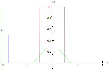
See also: [[Compton Imaging]] [[Parseval's Theorem]] # Convolution Motivation: Understanding the usage of a [[Point Spread Function]] when used in image reconstruction. ## Mathematical Definition A convolution is an integral that expresses the amount of overlap of one function $g$ as its shifted over another function $f$ [^1]. It is a [[Linear Shift-Invariant Systems|Linear Shift-Invariant operation]], which is very useful for signal analysis. Therefore you can say that it "blends" two functions together. I like to think of it like having one function slide across another function and consider the amount of overlap there is between them, and then plot that. [^1]: https://mathworld.wolfram.com/Convolution.html $[f*g](t) \equiv \int_0^t f(\tau)g(t-\tau) d\tau $ where $[f*g](t)$ denotes a convolution of $f$ and $g$. Convolution is more commonly taken across an infinite range. This is especially helpful for most of the times this operation is done on functions that are localized about a point, and rarely extend out to infinity. For example, the easiest way to visualize the function would be to define $f$ as a Boxcar function (two Heaviside step functions defined on [a, b]), and $g$ as the Dirac Delta function, $\delta(t)$ on $(-\infty, \infty)$. $\left[\Pi_{a,b}(t)*\delta(t) \right](t) = \int_{-\infty}^\infty \Pi_{a,b}(\tau)\delta(t-\tau) $ Since the Boxcar Function is defined to be 1 on [a, b], the result of this integral will be whatever the area of this boxcar function is measured to be over the range. In this case, it should be simply $(b-a) \times 1$ or, more simply, $b-a$. Here is a gif from Wolfram Mathworld that might help visualize it a bit:  It should also be noted that these concepts easily extend from 1D to ND space. ## Properties of Convolution Convolutions are: - Commutative: $(f_1 * f_2) (x) = (f_2 * f_1) (x)$ - Associative: $[(f_1 * f_2) *f_3] (x) = [f_1 * (f_2 *f_3)] (x)$ - Distributive: $[f_1 * (f_2 + f_3)](x) = (f_1 *f_2)(x) + (f_1 *f_3)(x)$ These mathematical properties are useful for studying Fourier Transforms [^2]. [^2]: Notes from MP573 Lecture 3 taught by Diego Hernando and Sean Fain ## Deconvolution The inverse operation of convolution, deconvolution is "ill-posed" and will not always yield a unique solution, even in the absence of noise. These involve using various filters, like a Weiner Filter or an inverse filter ## Convolution Theorem For any [[Fourier Transform]] pairs $f_1(x) / \hat{f}_1(u)$ and $f_2(x) / \hat{f}_2(u)$, the convolution of $f_1$ and $f_2$, $f_3(x) = [f_1 * f_2](x)$ has the Fourier Transform given by $ \hat{f}_3(u) = \hat{f}_1(u) \cdot \hat{f}_2(u) $ Or in other words, the convolution in the time domain is equivalent to multiplication in the frequency domain. It is also true to say that multiplication in the time domain is equivalent to convolution in the frequency domain.